9.1 K-means Clustering
Let we have a data set ${X_1,X_2,…,X_N}$ consisting of $N$ observations of random $D-$ dimensional Euclidean variable $X$. Our goal is to partition the data set into some number $K$ of clusters. Let the cluster $k$ is represented by a $D-$ dimensional vector $\mu_k$ where $k=1,2,…,K$. Our goal is then the assignment of data points to clusters and find the set of vectors ${\mu_k}$ such that the sum of the squares of the distanaces of each data point to its closets vector $\mu_k$ (or from the center of the assigned cluster), is a minimum.
For each data point $X_n$, a set binary indicator variables $r_{nk}$ where $k=1,2,…,K$ is introduced which encodes in which of the clustre the data point $X_n$ lies. If the data point $X_n$ is assigned to cluster $k$, $r_{nk} = 1$ and $r_{nj} = 0$ for all $j \neq k$. This is called as $1-of-K$ encoding scheme. An objective function called as distrortion measure can be defined as
$$\begin{align} J = \sum_{n=1}^N \sum_{k=1}^K r_{nk} ||X_n - \mu_k||^2 \end{align}$$
The goal is to find values of ${r_{nk}}$ and ${\mu_k}$ which minimize $J$. This can be done iteratively. In the first phase, we minimize $J$ with respect to $r_{nk}$, keeping $\mu_k$ fixed. In the second phase, we minimize $J$ with respect to $\mu_k$, keeping $r_{nk}$ fixed. These two-stages are repeated until convergence. These two stages correspond to the $E$ (expectation) and $M$ (maximization) steps of the $EM$ algorithm.
Determination of $r_{nk}$ for fixed value of $\mu_k$ takes a closed form solution as the term involving different $n$ are independent and hence for each $n$, $r_{nk}$ is chosen to be $1$ for whichever value of $k$ gives the minimum value of $||X_n - \mu_k||^2$. This means
$$\begin{align} r_{nk} = \begin{cases} 1, & \text{if } k=\arg \min_{j} ||X_n - \mu_j||^2\ 0, & \text{otherwise} \end{cases} \end{align}$$
Optimization of $\mu_k$ when $r_{nk}$ is kept fixed can be done by setting the derivative of $J$ with respect to $\mu_k$ to $0$. This gives us
$$\begin{align} 2\sum_{n=1}^N r_{nk} (X_n - \mu_k) = 0 \end{align}$$
$$\begin{align} \mu_k = \frac{\sum_n r_{nk}X_n}{\sum_n r_{nk}} \end{align}$$
The denominator is the number of points assigned to cluster $k$ and hence this expression simply means that the value of $\mu_k$ is the mean of the data points $X_n$ assigned to the cluster $k$. It should be noted that the convergence of the algorithm is assured but it may converge to local minima. The convergence speed and solution of the $K$-means algorithm depends on the choice of cluster means. A good initialization procedure is to choose the cluster centres $\mu_k$ to be equal to a random subset of $K$ data points.
A direct implementation of the $K$-means algorithm as discussed here can be relatively slow, because in each $E$ step it is necessary to compute the Euclidean distance between every prototype vector and every data point. So far, we have considered the batch version of the algorithm where the entire data set is used to update the cluster means. The on-line version of stochastic algorithm uses sequential update in which, for each data point $X_n$, we update the nearest prototype $\mu_k$ using
$$\begin{align} \mu_k^{new} = \mu_k^{old} + \eta_n(X_n - \mu_k^{old}) \end{align}$$
$\eta_n$ is the learning rate parameter which is made to decrease monotonically as more data points are considered. $K$-means algorithm is based on the use of squared Euclidean distance as the measure of dissimilarity. This limits the type of data variables which can be used and determination of the cluster means non-robust to outliers.
The $K$-means algorithm can be generalized by introducing a more general dissimilarity measure $\Gamma(X, X^{’})$ between two vectors $X$ and $X^{’}$ ane then minimizing the following distance measure
$$\begin{align} \tilde{J} = \sum_{n=1}^N \sum_{k=1}^K r_{nk} \Gamma(X_n, \mu_k) \end{align}$$
This is known as $K$-medoids algorithm. For a general choice of dissimilarity measure, the $M$-step is potentially more complex and hence it is common to restrict each cluster prototype to one of the data points in the cluster. This allows the algorithm to be implemented for any choice of dissimilarity measure as long as it can be readily evaluated. One of the notable feature of the $K$-means algorithm is that at each iteration, every data point is assigned uniquely to one and only one of the clusters. Algorithms which use soft assignment of points are also present.
9.1.1 Image Segmentation and Compression
The goal of image segmentation is to partition an image into regions each of which has reasonably homogeneous visual appearance. The image space is not Euclidean. The $K$-means algorithm can be applied to the image where for a given value of $K$, the image is represented using a palette of only $K$ colours.
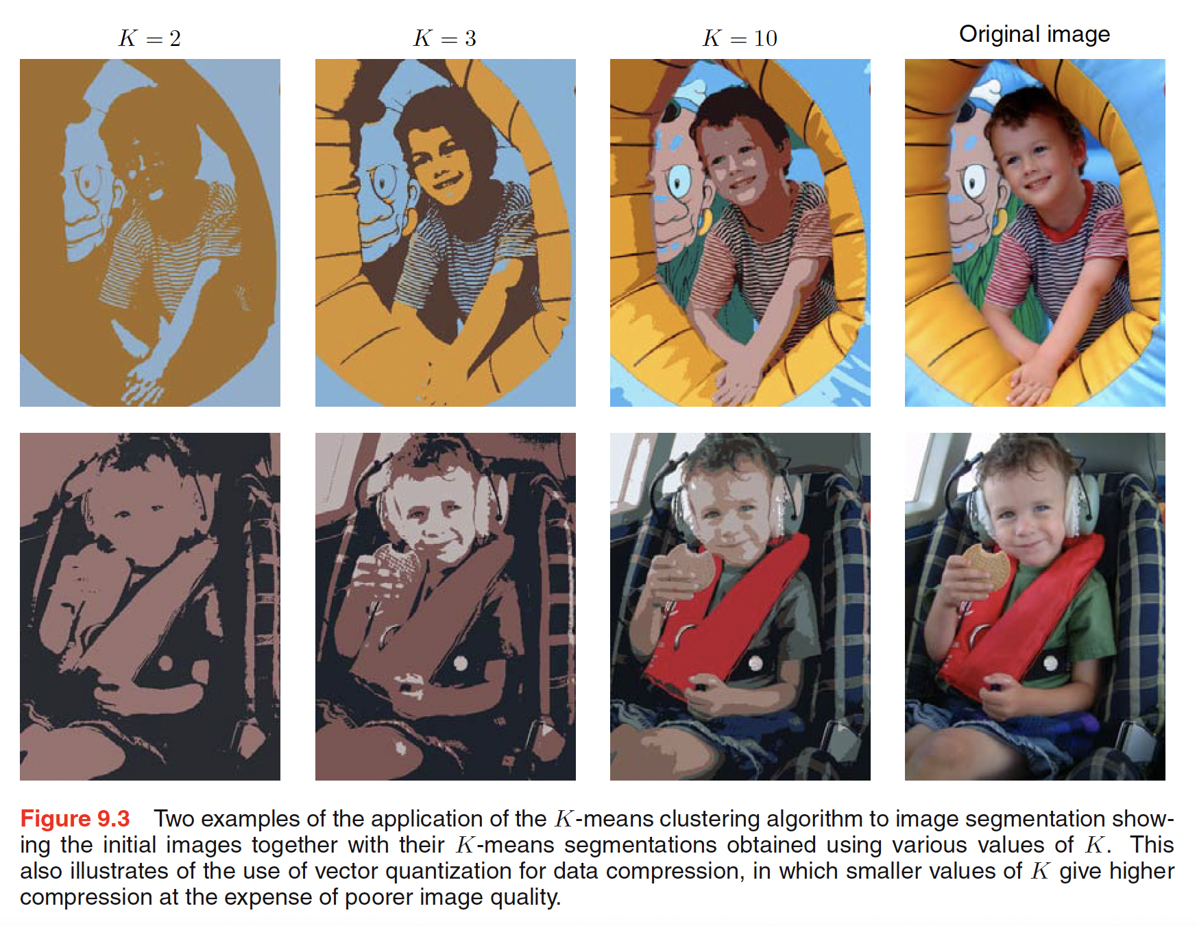
It is important to distinguish between lossless data compression, in which the goal is to be able to reconstruct the original data exactly from the compressed representation, and lossy data compression, in which we accept some errors in the reconstruction in return for higher levels of compression than can be achieved in the lossless case.
Lossy data compression can be achieved using $K$-means algorithm. For each data point the cluster to which it is assigned and for each cluster, the cluster mean is stored. Each data point is then approximated by its nearest cluster mean $\mu_k$. This saves a lot of space for $K « N$ and results in higher level of compression.