8.4.4 The Sum-product Algorithm
Let us assume that all the variables in a model are discrete and hence marginalization corresponds to performing sums. To use the same algorithm for all kind of graphs, we first convert the original graph into a factor graph so that we can deal with both directed and undirected model using the same framework. To find the marginal distribution $p(x)$ for a particular variable node $x$, we need to sum the joint distribution over all variables except $x$ so that
$$\begin{align} p(x) = \sum_{X/\ x}p(X) \end{align}$$
where $X/\ x$ denotes the set of all the variables in $X$ except $x$. Now we can substitute for $p(X)$ using the factor graph equation and then inerchange the summations and products to get an efficient algorithm. The joint distribution can be written as
$$\begin{align} p(X) = \prod_{s \in ne(x)} F_s(x,X_s) \end{align}$$
where $ne(x)$ is the set of factor nodes that are neighbours of $x$. $X_s$ denotes the set of all variable nodes in the subtree connected to the variable node $x$ via the factor node $f_s$. $F_s(x,X_s)$ represents all the factors in the group associated with factor node $f_s$. Substituting the value of $p(X)$ in the equation to evaluate the marginal distribution, we have
$$\begin{align} p(x) = \sum_{X/\ x} \prod_{s \in ne(x)} F_s(x,X_s) = \sum_{X_s} \prod_{s \in ne(x)} F_s(x,X_s) \end{align}$$
$$\begin{align} p(x) = \prod_{s \in ne(x)} \sum_{X_s} F_s(x,X_s) \end{align}$$
$$\begin{align} p(x) = \prod_{s \in ne(x)} \mu_{f_s \to x} (x) \end{align}$$
where the set of functions $\mu_{f_s \to x} (x)$ is defined as
$$\begin{align} \mu_{f_s \to x} (x) = \sum_{X_s} F_s(x,X_s) \end{align}$$
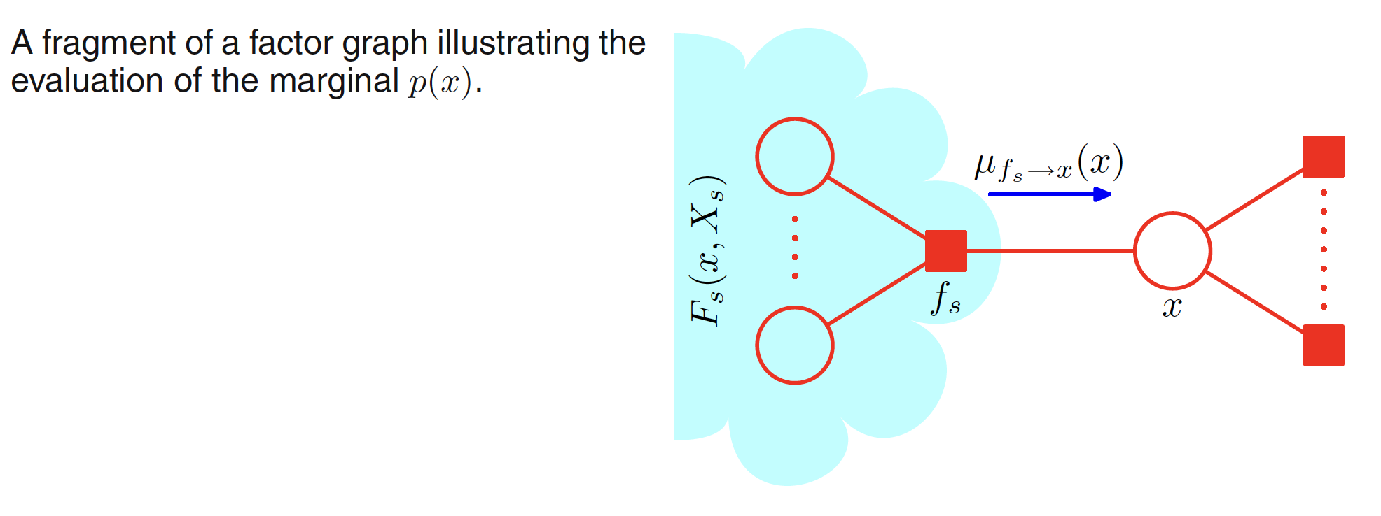
It can be viewed as messages from the factor node $f_s$ to the variable node $x$. The required marginal $p(x)$ is the product of all the incoming messages arriving at the variable node $x$. The flow of these messages is shown in the below figure.
First of all let the other variables associated with factor $f_s$ apart from $x$ be $x_1,x_2,…,x_M$. This is illustrated in below figure. This means that the set of variables ${x,x_1,x_2,…,x_M}$ are the variables on which the factor $f_s$ depends and hence it can be denoted using $X_s$. As shwon in the below figure, for each factor node, we will have incoming messages from the adjacent variable nodes, which is $\mu_{x_M \to f_s} (x_M)$ for the message passed from variable node $x_M$ to factor node $f_s$.
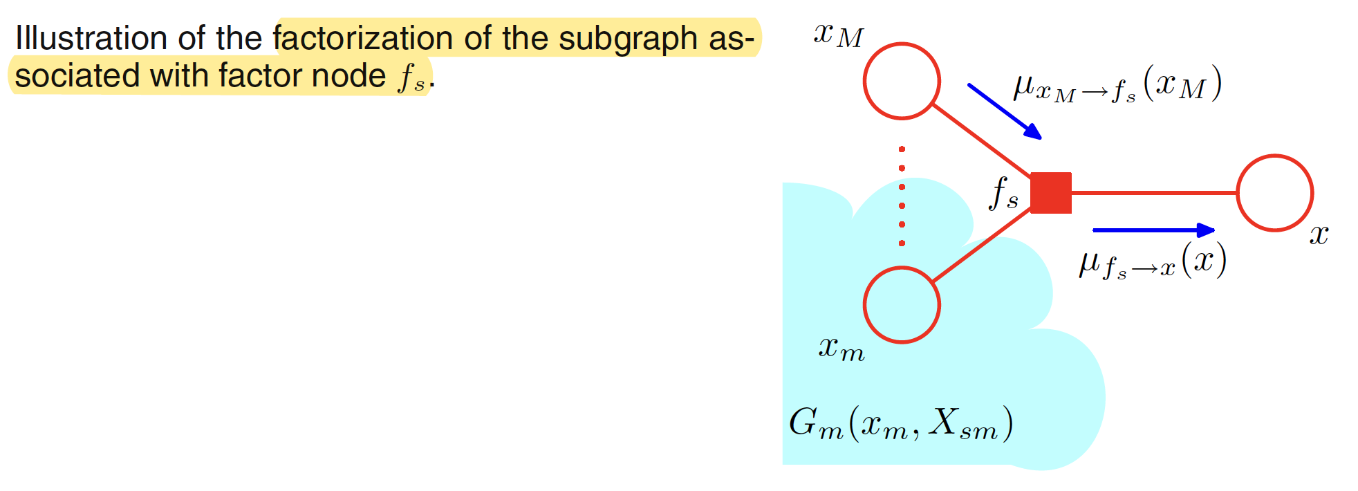
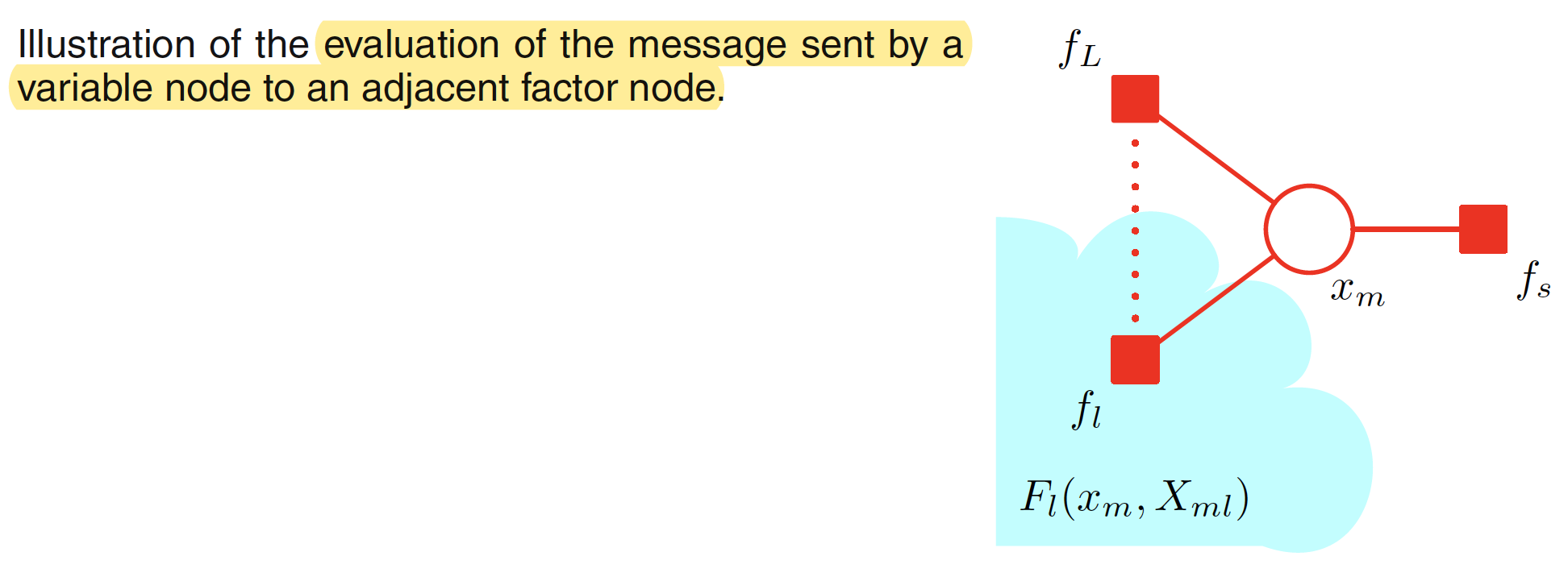
Now, let us dive deep into the view with respect to the variable nodes. First of all, as $F_s(x,X_s)$ is associated with the factor node $f_s$, we have a similar function associated with each of the variable nodes and is denoted by $G_m(x_m,X_{sm})$ for variable node $x_m$. This is illustrated in following figure. The term $G_m(x_m,X_{sm})$ will depend on all the other factor nodes linked to $x_m$ apart from $f_s$ and will be given as
$$\begin{align} G_m(x_m,X_{sm}) = \prod_{l \in ne(x_m)/ f_s} F_l(x_m,X_{ml}) \end{align}$$
The product is taken over all the neighbouring factor nodes of $x_m$ apart from $f_s$.
Now, each factor $F_s(x,X_s)$ is described as
$$\begin{align} F_s(x,X_s) = f_s(x,x_1,…,x_M)G_1(x_1,X_{s1})…G_M(x_M,X_{sM}) \end{align}$$
which is illustrated in the second figure. Apart from this, message from variable nodes to factor nodes can be evaluated as
$$\begin{align} \mu_{x_m \to f_s} (x_m) = \sum_{X_{sm}} G_m(x_m,X_{sm}) \end{align}$$
Combining these, we have
$$\begin{align} \mu_{f_s \to x} (x) = \sum_{X_s} F_s(x,X_s) = \sum_{X_s} f_s(x,x_1,…,x_M)G_1(x_1,X_{s1})…G_M(x_M,X_{sM}) \end{align}$$
$$\begin{align} = \sum_{X_s} \bigg[f_s(x,x_1,…,x_M) \prod_{m \in ne(f_s)/\ x} G_m(x_m,X_{sm}) \bigg] \end{align}$$
$$\begin{align} = \bigg[ \sum_{X_s} f_s(x,x_1,…,x_M) \bigg] \bigg[ \prod_{m \in ne(f_s)/\ x} \sum_{X_s} G_m(x_m,X_{sm}) \bigg] \end{align}$$
As $X_s={x_1,x_2,…,x_M}$, which are the variable nodes connected to $f_s$ apart from $x$, the above expression can be re-written as
$$\begin{align} \mu_{f_s \to x} (x) = \sum_{x_1}…\sum_{x_M} f_s(x,x_1,…,x_M) \prod_{m \in ne(f_s)/\ x} \bigg[ \sum_{X_{sm}} G_m(x_m,X_{sm}) \bigg] \end{align}$$
$$\begin{align} = \sum_{x_1}…\sum_{x_M} f_s(x,x_1,…,x_M) \prod_{m \in ne(f_s)/\ x} \mu_{x_m \to f_s} (x_m) \end{align}$$
Hence, to evaluate the message sent by a factor node to a variable node along the link connecting them, take the product of the incoming messages $\mu_{x_m \to f_s} (x_m)$ along all other links (from the connected variable nodes) coming into the factor node, multiply by the factor $f_s(x,x_1,…,x_M)$ associated with that node, and then marginalize over all of the variables $X_s={x_1,x_2,…,x_M}$ associated with the incoming messages.
Finally the message passed from the variable node to factor node $\mu_{x_m \to f_s} (x_m)$ can be evaluated as
$$\begin{align} \mu_{x_m \to f_s} (x_m) = \sum_{X_{sm}} G_m(x_m,X_{sm}) \end{align}$$
Substituting the expression for $G_m(x_m,X_{sm})$, we have
$$\begin{align} \mu_{x_m \to f_s} (x_m) = \sum_{X_{sm}} \prod_{l \in ne(x_m)/ f_s} F_l(x_m,X_{ml}) = \prod_{l \in ne(x_m)/ f_s} \sum_{X_{ml}} F_l(x_m,X_{sm}) \end{align}$$
$$\begin{align} \mu_{x_m \to f_s} (x_m) = \prod_{l \in ne(x_m)/ f_s} \mu_{f_l \to x_m} (x_m) \end{align}$$
This means that to evaluate the message sent by a variable node to a factor node, we take the product of the incoming messages along the other links (all the other factor nodes connected to that variable node). A variable node can send a message to the factor node once it has received the incoming mesagges from all the adjacent factor nodes.
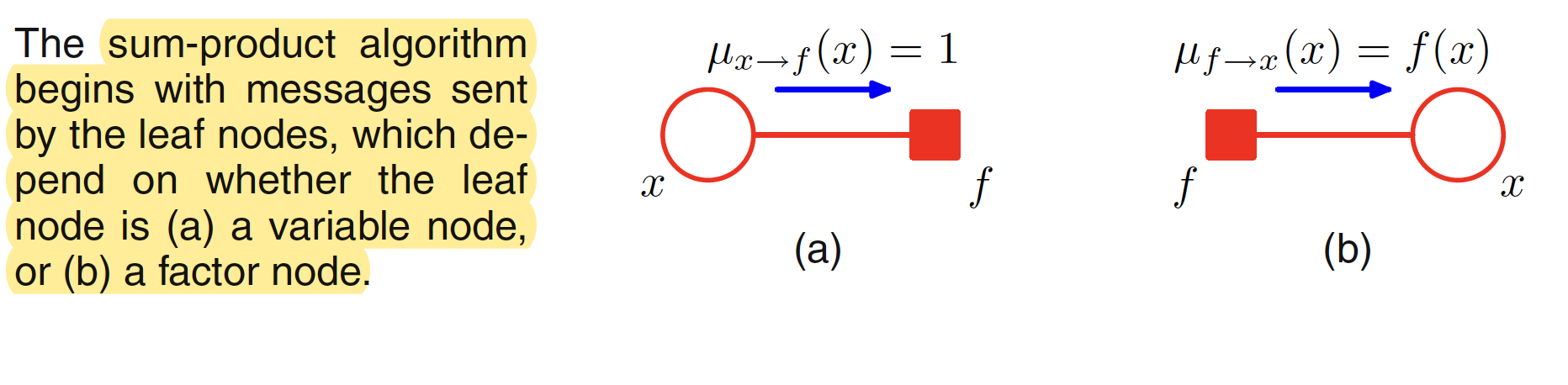
To calculate the marginal at variable node $x$, we can view the node as $x$ the root of the tree and begin computing the messages recursively from the leaf nodes. If a leaf node is a variable node, the message it sends along its one and only link is given by
$$\begin{align} \mu_{x \to f} (x) = 1 \end{align}$$
If the leaf node is a factor node, the message sent will take the form
$$\begin{align} \mu_{f \to x} (x) = f(x) \end{align}$$
This is illustrated in below figure.
Once we have computed the messages passed by the leaf nodes, the message passing step for other variable and factor nodes are computed recursively until we reach the root node $x$. Each node can send a message towards the root once it has received the messages from all of its neighbours. Once the root node $x$ has received the message from all of its neighbours, the required marginal can be evaluated by summing the messages over.
The marginal $p(X_s)$ associated with the set of nodes at the factor node $f_s$ is the product of messages arriving at the factor node and the local factor at the node and is givne as
$$\begin{align} p(X_s) = f_s(X_s) \prod_{i \in ne(f_s)} \mu_{x_i \to f_s} (x_i) \end{align}$$
Let us consider an example to demonstrate the sum-product algorithm using the following graph.
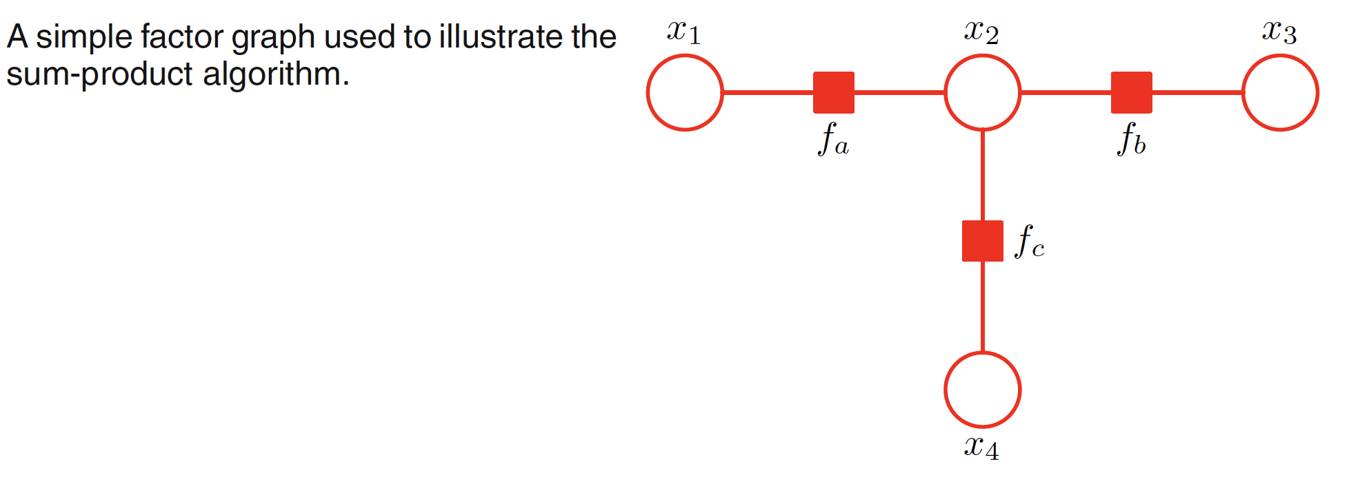
The unnormalized joint distribution of the above graph is given as
$$\begin{align} \tilde{p}(X) = f_a(x_1,x_2)f_b(x_2,x_3)f_c(x_2,x_4) \end{align}$$
Let $x_3$ be the root node. This makes $x_1, x_2$ as two leaf nodes. Leaf nodes being variable nodes, the messages from the leaf nodes are shown below.
$$\begin{align} \mu_{x_1 \to f_a} (x_1) = 1 \end{align}$$
$$\begin{align} \mu_{x_4 \to f_c} (x_4) = 1 \end{align}$$
Now we will evaluate the messages flowing from the factor nodes $f_a,f_c$ towards variable node $x_2$. As we know that the message flowing from a factor node to a variable node is given by the product of the incoming messages from the connected variable nodes coming into the factor node, multiplied by the factor associated with the node, finally marginalized over all of the variables associated with the incoming messages. Hence the messages are given as:
$$\begin{align} \mu_{f_a \to x_2} (x_2) = \sum_{x_1} f_a(x_1,x_2) \mu_{x_1 \to f_a} (x_1) = \sum_{x_1} f_a(x_1,x_2) \end{align}$$
$$\begin{align} \mu_{f_c \to x_2} (x_2) = \sum_{x_4} f_c(x_2,x_4) \mu_{x_4 \to f_c} (x_4) = \sum_{x_4} f_c(x_2,x_4) \end{align}$$
Then, we have to evaluate the message flowing from variable node $x_2$ to the factor node $f_b$. The message sent by a variable node to a factor node is the product of the incoming messages along the factor nodes connected to the variable node. This gives us
$$\begin{align} \mu_{x_2 \to f_b} (x_2) = \mu_{f_a \to x_2} (x_2) \mu_{f_c \to x_2} (x_2) \end{align}$$
Finally, the message form the factor node $f_b$ to the variable root node $x_3$ is given as
$$\begin{align} \mu_{f_b \to x_3} (x_3) = \sum_{x_2} f_b(x_2,x_3) \mu_{x_2 \to f_b} (x_2) \end{align}$$
Similarly, the message propagated from the root node $x_3$ towards the leaf nodes can be evaluated as:
$$\begin{align} \mu_{x_3 \to f_b} (x_3) = 1 \end{align}$$
$$\begin{align} \mu_{f_b \to x_2} (x_2) = \sum_{x_3} f_b(x_2,x_3) \end{align}$$
$$\begin{align} \mu_{x_2 \to f_a} (x_2) = \mu_{f_b \to x_2} (x_2) \mu_{f_c \to x_2} (x_2) \end{align}$$
$$\begin{align} \mu_{x_2 \to f_c} (x_2) = \mu_{f_b \to x_2} (x_2) \mu_{f_a \to x_2} (x_2) \end{align}$$
$$\begin{align} \mu_{f_a \to x_1} (x_1) = \sum_{x_2} f_a(x_1,x_2) \mu_{x_2 \to f_a} (x_2) \end{align}$$
$$\begin{align} \mu_{f_c \to x_4} (x_4) = \sum_{x_2} f_a(x_2,x_4) \mu_{x_2 \to f_c} (x_2) \end{align}$$
Finally, the marginal at any of the variable node can be comupted as
$$\begin{align} p(x) = \prod_{s \in ne(x)} \mu_{f_s \to x} (x) \end{align}$$
Using this, the marginal at node $x_2$ is given as
$$\begin{align} p(x_2) = \mu_{f_a \to x_2} (x_2) \mu_{f_b \to x_2} (x_2) \mu_{f_c \to x_2} (x_2) \end{align}$$
$$\begin{align} = \bigg[\sum_{x_1}f_a(x_1,x_2)\bigg] \bigg[\sum_{x_3}f_b(x_2,x_3)\bigg] \bigg[\sum_{x_4}f_c(x_2,x_4)\bigg] \end{align}$$
$$\begin{align} = \sum_{x_1}\sum_{x_3}\sum_{x_4}f_a(x_1,x_2)f_b(x_2,x_3)f_c(x_2,x_4) \end{align}$$
$$\begin{align} = \sum_{x_1}\sum_{x_3}\sum_{x_4} \tilde{p}(X) \end{align}$$
which comes out to be as desired.
8.4.5 The Max-Sum Algorithm
The max-sum algorithm can be viewed as the application of dynamic programming in the context of graphical models. In practice, we usually want to find the value the set of variables (represented by a vector $X^{max}$) which maximizes the joint distribution, such that
$$\begin{align} X^{max} = \arg \max_{X} p(X) \end{align}$$
for which the corresponding value of the joint probability will be given as
$$\begin{align} p(X^{max}) = \max_{X} p(X) \end{align}$$
Breaking down the $X$ of the max operator into its components, we have
$$\begin{align} \max_{X} p(X) = \max_{x_1}…\max_{x_M} p(X) \end{align}$$
where $M$ is the total number of variables. Before proceeding further, it is worthwhile to state one of the properties of max operator. If $a \geq 0$, then
$$\begin{align} \max (ab,ac) = a \max (b,c) \end{align}$$
Let’s try to decompose the evaluation of the probability maximum for the case of chain of nodes example. The evaluation of probability maximum can be written as
$$\begin{align} \max_X p(X) = \frac{1}{Z} \max_{x_1}…\max_{x_N} \bigg[\Psi_{1,2}(x_1,x_2)…\Psi_{N-1,N}(x_{N-1},x_N)\bigg] \end{align}$$
$$\begin{align} \frac{1}{Z} \max_{x_1}\bigg[\Psi_{1,2}(x_1,x_2)\bigg[…\max_{x_N}\Psi_{N-1,N}(x_{N-1},x_N)\bigg]\bigg] \end{align}$$
Exchanging the max and product operator gives us a much more simpler problem to solve. One of the major problem which is faced while solving the maximization problem is that the product of many small probabilities can lead to numerical underflow problem and hence it is convinient to work with the logarithmic function. The logarithm is a monotonic function, i.e. if $a > b$ then $\ln a > \ln b$. This means that the max operator and the logarithmic function can be interchanged, so that
$$\begin{align} \ln \bigg( \max_{X} p(X) \bigg) = \max_{X} \ln p(X) \end{align}$$
The distributive property is also preserved as
$$\begin{align} \max(a+b,a+c) = a + \max(b,c) \end{align}$$
Hence, taking algorithm will simply has the effect of replacing the products in the max-product algorithm with sums which gives us the max-sum algorithm.