9.2 Mixtures of Gaussians
This section describes the formulation of Gaussian mixtures in terms of discrete latent variables. The gaussian mixture distribution can be written as a linear superposition of Gaussian in the form
$$\begin{align} p(X) = \sum_{k=1}^{K} \pi_k N(X|\mu_k, \Sigma_k) \end{align}$$
Let us introduce a $K-$ dimensional binary random variable $z$ having a $1-of-K$ representation in which a particular element $z_k$ satisfies $z_k \in {0,1}$ and $\sum_k z_k = 1$. The joint distribution $p(X,z)$ can then be represented in terms of the marginal distribution $p(z)$ and conditional distribution $p(X|z)$. The marginal distribution is given as
$$\begin{align} p(z_k = 1) = \pi_k \end{align}$$
where the parameter $\pi_k$ must satisfy $0 « \pi_k « 1$ and $\sum_k \pi_k = 1$. This marginal distribution can also be written as
$$\begin{align} p(z) = \prod_{k=1}^{K} \pi_k^{z_k} \end{align}$$
The conditional distribution of $X$ given a particular value of $z$ is a Gaussian and can be given as
$$\begin{align} p(X|z_k = 1) = N(X|\mu_k, \Sigma_k) \end{align}$$
which can also be written in the form
$$\begin{align} p(X|z) = \prod_{k=1}^{K} N(X|\mu_k, \Sigma_k)^{z_k} \end{align}$$
The joint distribution $p(X,z)$ is given as $p(z)p(X|z)$ and the marginal distribution $p(X)$ can be computed as
$$\begin{align} p(X) = \sum_{z}p(X,z) = \sum_{z}p(z)p(X|z) = \sum_{k=1}^{K} \pi_k N(X|\mu_k, \Sigma_k)^{z_k} \end{align}$$
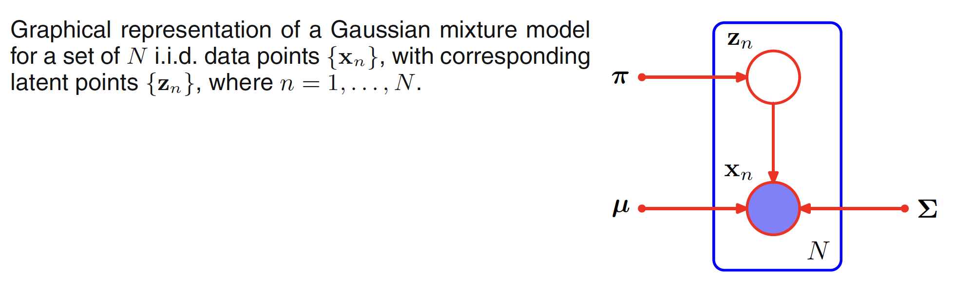
It should be noted that for every observed data point $X_n$ we have a corresponding latent variable $z_n$.
Another quantity which plays an important role is $\gamma(z_k)$ which denotes $p(z_k = 1 | X)$, whose value can be found using Bayes theorem as
$$\begin{align} \gamma(z_k) = p(z_k = 1 | X) = \frac{p(z_k=1)p(X|z_k=1)}{p(X)} \end{align}$$
$$\begin{align} = \frac{p(z_k=1)p(X|z_k=1)}{\sum_z p(X,z)} \end{align}$$
$$\begin{align} = \frac{p(z_k=1)p(X|z_k=1)}{\sum_z p(z)p(X|z)} \end{align}$$
$$\begin{align} = \frac{p(z_k=1)p(X|z_k=1)}{\sum_{j=1}^{K} p(z_j=1)p(X|z_j=1)} \end{align}$$
$$\begin{align} = \frac{\pi_k N(X|\mu_k, \Sigma_k)}{\sum_{j=1}^{K} \pi_j N(X|\mu_j, \Sigma_j)} \end{align}$$
$\pi_k$ can be viewed as the prior probability of $z_k =1$ and $\gamma(z_k)$ as the posterior probability once we have observed $X$. $\gamma(z_k)$ is also called as responsibility that component $k$ takes for explaining the observation $X$.
9.2.1 Maximum Likelihood
Let the data points ${X_1, X_2,…, X_N}$ be represented as a $N \times D$ matrix $X$ where $n^{th}$ row of the matrix is $X_N^T$. Let the latent varibales are representead as $N \times K$ matrix $Z$ where $n^{th}$ row of the matrix is $z_N^T$. If we assume that the data points are drawn indeoendently from the distribution, then the Gaussian mixture model for this i.i.d. data set will be represented as below.
As we know that the Gaussian mixture distribution for individual data point is represented as
$$\begin{align} p(X_n) = \sum_{k=1}^{K} \pi_k N(X_n|\mu_k, \Sigma_k) \end{align}$$
For $N$ i.i.d. data points, the likelihood function can then be modeled as
$$\begin{align} p(X|\pi, \mu, \Sigma) = \prod_{n=1}^{N} \sum_{k=1}^{K} \pi_k N(X_n|\mu_k, \Sigma_k) \end{align}$$
Taking logarithm, we get the log likelihood function as
$$\begin{align} \ln p(X|\pi, \mu, \Sigma) = \sum_{n=1}^{N} \ln \bigg[\sum_{k=1}^{K} \pi_k N(X_n|\mu_k, \Sigma_k) \bigg] \end{align}$$
Let one of the components of mixture model has its mean exactly equal to one of the data points, i.e. $\mu_j = X_n$. This data point will contribute a term in the likelihood function of the form (exponential term vanishes as $\mu_j = X_n$)
$$\begin{align} N(X_n|\mu_j, \sigma_j^2I) = \frac{1}{(2\pi)^{1/2}}\frac{1}{\sigma_j} \end{align}$$
If we consider the limit $\sigma_j \to 0$, the above term goes to infinity and hence the log likelihood function will also go to infinity. Hence, in case of signiularity (when one of the Gaussian components collapses to a specific data point), the maximization of log likelihood function is not a well posed problem. This problem of singularity can be avoided by detecting when a Gaussian component is collapsing and resetting its mean to a randomly chosen value while also resetting its covariance to some large value, and then continuing with the optimization.
Maximizing the log likelihood function for a Gaussian mixture model turns out to be a more complex problem than for the case of a single Gaussian. The difficulty arises from the presence of the summation over $k$ that appears inside the logarithm. The logarithm function does not act directly on the Gaussian and hence there doesn’t exist a closed form solution.
9.2.2 EM for Gaussian Mixtures
Expectation-maximization algorithm can be used to find the maximum likelihood solutions for models with latent variables. Let us start with the log likelihood function of Gaussian mixture model.
$$\begin{align} \ln p(X|\pi, \mu, \Sigma) = \sum_{n=1}^{N} \ln \bigg[\sum_{k=1}^{K} \pi_k N(X_n|\mu_k, \Sigma_k) \bigg] \end{align}$$
Taking the derivative of above expression w.r.t. $\mu_k$ and setting it to 0, we have
$$\begin{align} - \sum_{n=1}^{N} \frac{\pi_k N(X_n|\mu_k,\Sigma_k)}{\sum_{j}\pi_j N(X_n|\mu_j,\Sigma_j)} [\Sigma_k(X_n - \mu_k)] = 0 \end{align}$$
$$\begin{align} - \sum_{n=1}^{N} \gamma(z_{nk}) [\Sigma_k(X_n - \mu_k)] = 0 \end{align}$$
Solving this equation, we have
$$\begin{align} \mu_k = \frac{\sum_{n=1}^N \gamma(z_{nk}X_n)}{\sum_{n=1}^N \gamma(z_{nk})} = \frac{\sum_{n=1}^N \gamma(z_{nk}X_n)}{N_k} \end{align}$$
where
$$\begin{align} N_k = \sum_{n=1}^N \gamma(z_{nk}) \end{align}$$
$N_k$ can be interpretted as the effective number of points assigned to cluster $k$. The mean $\mu_k$ for the $k^{th}$ Gaussian component is obtained by taking a weighted mean of all the points in the data set, where the weighing factor for data point $X_n$ is given by the posterior probability $\gamma(z_{nk})$ that component $k$ was responsible for generating $X_n$. The rest of the parameters can be obtained using similar technique and are given as
$$\begin{align} \Sigma_k = \frac{1}{N_k}\sum_{n=1}^N \gamma(z_{nk}) (X_n - \mu_k)(X_n - \mu_k)^T \end{align}$$
$$\begin{align} \pi_k = \frac{N_k}{N} \end{align}$$
The above expression can be interpretted as the mixing coefficient of the $k^{th}$ component is given by the average responsibility which that component takes for explaining the data. It should be noted that these solutions are not the closed form solution for the mixture model as the responsibilities $\gamma(z_{nk})$ depend on those parameters. A simple iterative scheme can be used to find the values for these parameters. We first choose some initial values for the means, covariances and mixing coefficients and then we alternate between E and M steps. In the expectation step (E step), we use the current values for the parameters to evaluate the responsibilities $\gamma(z_{nk})$. These updated responsibilities can then be used to re-estimate the means, covariances and mixing-coefficients in the maximization step. Each update to the parameters resulting from an E step followed by an M step is guaranteed to increase the log likelihood function. In practice, the algorithm is deemed to have converged when the change in the log likelihood function, or alternatively in the parameters, falls below some threshold. The EM-algorithm for the mixture model applied on a data set is shown in below figure.
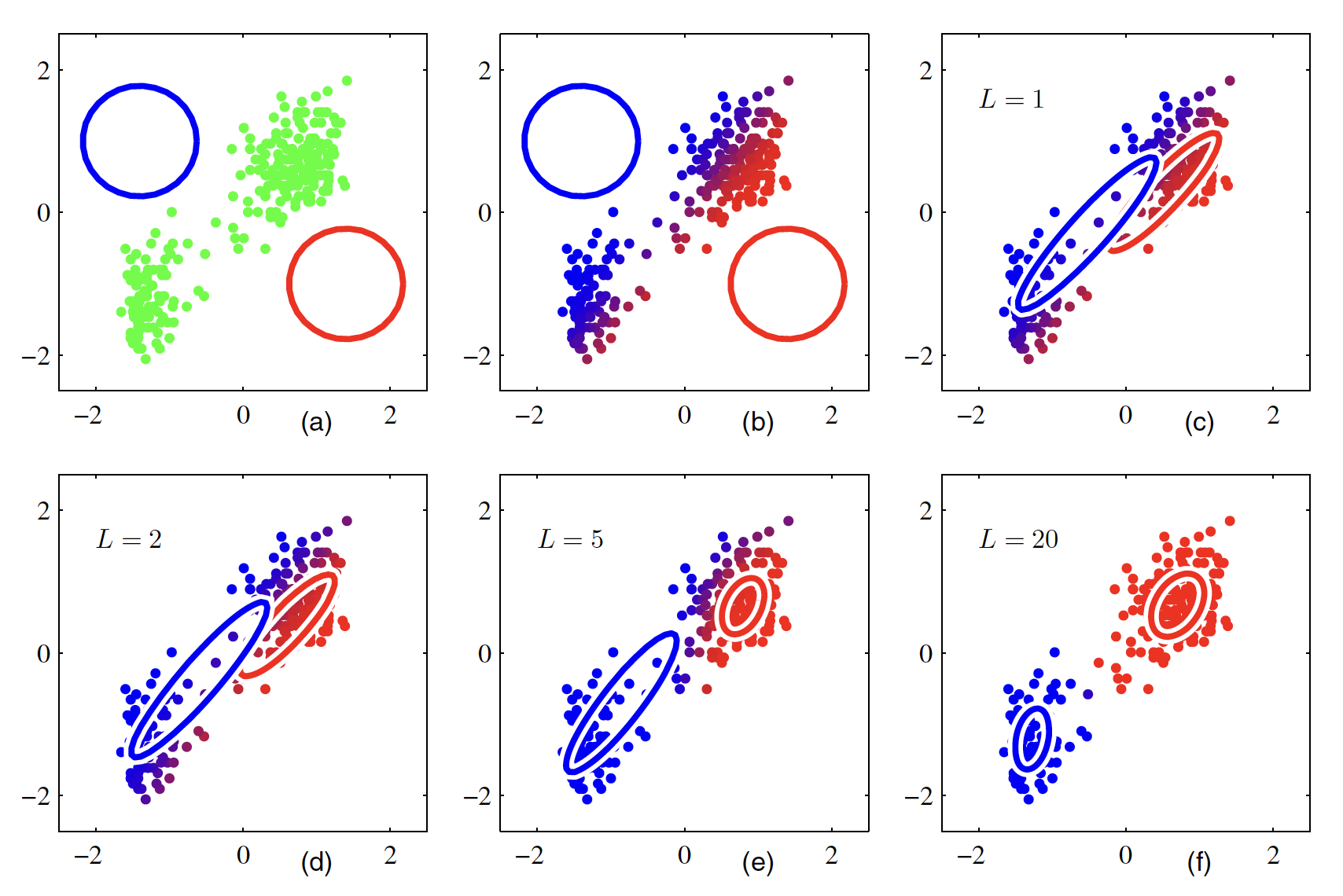
Gaussian components are shown as blue and red circles. The blue and red component in the color of data points show how much contribution of blue and red Gaussian have in generation of those data points. Hence, the points which have significant probability of belonging to either cluster appear purple. The EM algorithm takes much more iterations and significant computation to converge comared to $K$-means. It is hence a good practice to initialize the means of the Gaussians using results of $K$-means algorithm. The covariance matrices can conveniently be initialized to the sample covariances of the clusters found by the K-means algorithm, and the mixing coefficients can be set to the fractions of data points assigned to the respective clusters.