8.4 Inference in Graphical Models
The problem of inference in graphical models, in which some of the nodes in a graph are clamped to the observed values, aims to compute the posterior distribution of one or more subset of nodes. The graphical structure can be exploited to find the efficient and transparent algorithms for inference. These algorithms usually can be expressed in terms of the propagation of local messages around the graph. Let us consider the graphical representation of Bayes theorem shown in the below figure.
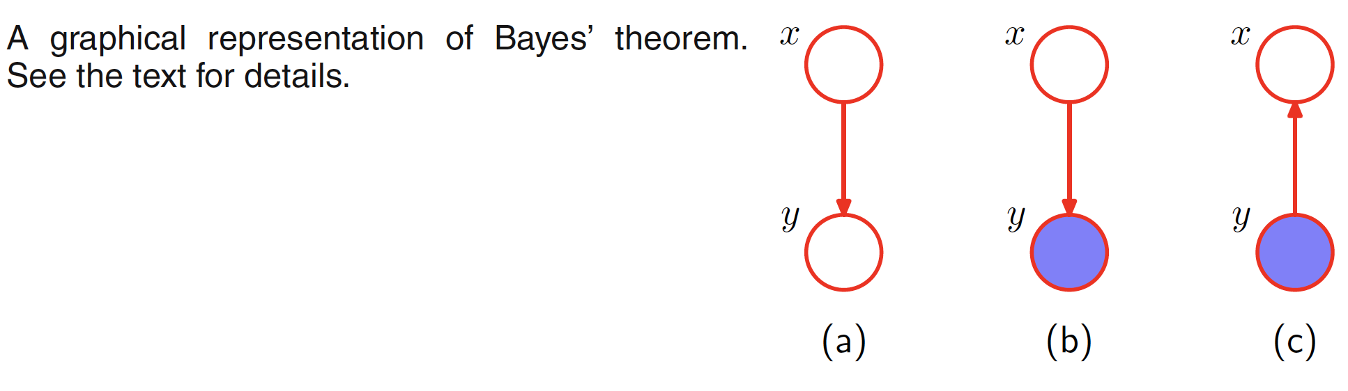
The joint distribution over two variables can be represented as $p(X,Y) = p(X)p(Y|X)$. This distribution is represented by the first figure. Given the marginal distribution $p(X)$, which can also be interpretted as a prior over the latent variable $X$, our goal is to infer the correspoding posterior distribution over $X$. This can be evaluated using Bayes’ theorem
$$\begin{align} p(X|Y) = \frac{p(X,Y)}{p(Y)} = \frac{p(X)p(Y|X)}{p(Y)} \end{align}$$
where $p(Y)$ can be evaluated by marginalizing $p(X,Y)$ over $X$.
8.4.1 Inference on a Chain
Consider an undirected graph which has $N$ nodes connected in a chain, i.e. node $X_i$ is connected to $X_{i-1}$ and $X_{i+1}$. The joint distribution for this graph takes the form
$$\begin{align} p(X) = \frac{1}{Z}\Psi_{1,2}(X_1,X_2)\Psi_{2,3}(X_2,X_3)…\Psi_{N-1,N}(X_{N-1},X_N) \end{align}$$
When each node represents a discrete varaible having $K$ states, the total number of parameters in the joint distribution will be $(N-1)K^2$, $K^2$ for each of the $N-1$ nodes. The marginal distribution for one of the node say $X_n$ can be found by summing the joint distribution (in case of discrete variables) over each node except $X_n$, which is
$$\begin{align} p(X_n) = \sum_{X_1}…\sum_{X_{n-1}}\sum_{X_{n+1}}…\sum_{X_N} p(X) \end{align}$$
Substituting the term for $p(X)$ and rearranging the summation, we can evaluate the marginal distribution for $X_n$ in a computational efficient way. The last summation (over $X_N$) will just include the potential $\Psi_{N-1,N}(X_{N-1},X_N)$ as this is the only term which depends on $X_N$ and hence following summation can be performed
$$\begin{align} \sum_{X_N} \Psi_{N-1,N}(X_{N-1},X_N) = f(X_{N-1}) \end{align}$$
Next summation will include the above function and the potential which depends on $X_{N-1}$ and will be given as
$$\begin{align} \sum_{X_{N-1}} \Psi_{N-2,N-1}(X_{N-2},X_{N-1})f(X_{N-1}) = f(X_{N-2}) \end{align}$$
It should be noted that as each summation effectivey removes a varaible from the distribution, this can be viewed as the removal of node from the graph. If we group the potential and summation this way, the marginal can be expressed as
$$\begin{align} p(X_n) = \frac{1}{Z}\bigg[\sum_{X_{n-1}} \Psi_{n-1,n}(X_{n-1},X_{n}) … \bigg[\sum_{X_{2}} \Psi_{2,3}(X_{2},X_{3})\bigg[\sum_{X_{1}} \Psi_{1,2}(X_{1},X_{2})\bigg]\bigg]\bigg] \end{align}$$
$$\begin{align} \bigg[\sum_{X_{n+1}} \Psi_{n,n+1}(X_{n},X_{n+1}) … \bigg[\sum_{X_{N-1}} \Psi_{N-2,N-1}(X_{N-2},X_{N-1})\bigg[\sum_{X_{N}} \Psi_{N-1,N}(X_{N-1},X_{N})\bigg]\bigg]\bigg] \end{align}$$
This can be further represented as the product of two factors times the normalization constant as
$$\begin{align} p(X_n) = \frac{1}{Z} \mu_{\alpha}(X_n) \mu_{\beta}(X_n) \end{align}$$
This can be interpretted as $\mu_{\alpha}(X_n)$ being the message passed forward along the chain from node $X_{n-1}$ to $X_n$. Similarly, $\mu_{\beta}(X_n)$ being the message passed backward along the chain from node $X_{n+1}$ to $X_n$. These messages can be computed recursively until we reach the desired node as shown in the below figure.
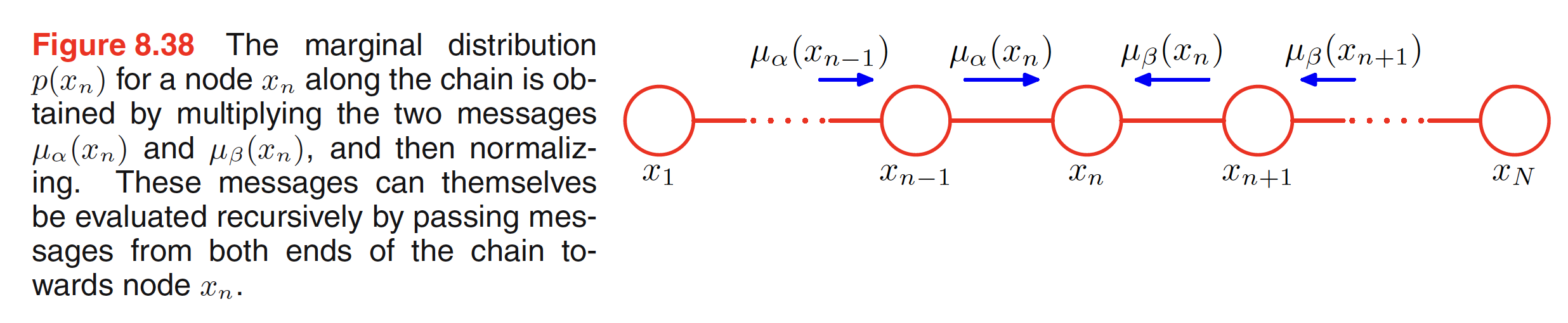
The outgoing message $\mu_{\alpha}(X_n)$ can be evaluated as follows:
$$\begin{align} \mu_{\alpha}(X_n) = \sum_{X_{n-1}} \Psi_{n-1,n}(X_{n-1},X_{n}) \bigg[\sum_{X_{n-2}} …\bigg] = \sum_{X_{n-1}} \Psi_{n-1,n}(X_{n-1},X_{n}) \mu_{\alpha}(X_{n-1}) \end{align}$$
This means that the outgoing message $\mu_{\alpha}(X_n)$ is obtained by multiplying the incoming message $\mu_{\alpha}(X_{n-1})$ with the local potential $\Psi_{n-1,n}(X_{n-1},X_{n})$ involving the node variable and the outgoing variable and then summing over the node variable. Graphs shown in above figure are called as Markov chains and the corresponding message passing equations are the example of Chapman-Kolmogorov equations.
8.4.2 Trees
In the previous section, we have seen that for a graph where nodes are in chain, exact inference can be performed efficiently in linear time wrt number of nodes using an algorithm that passes message along the chain. The same conecpt of local message passing can be used to perform the inference problem on another class of graphs called as trees.
In an undirected graph, a tree is defined as a graph in which there is one and only one path between pair of nodes. Such graphs do not have loops. In a directed graph, a tree is a graph which has a single root (node which does not have any parent), and all the other nodes have one parent. If a directed tree is converted into an undirected grapha, the moralization step will not add any links as all nodes have at most one parent and hence the corresponding moralized graph will be an undirected tree.
8.4.3 Factor Graphs
Let the joint distribution over a set of variables is written in the form of a product of factors as
$$\begin{align} p(X) = \prod_{s} f_s(X_s) \end{align}$$
where $X_s$ denots a subset of the variables. The joint distribution for directed and undirected graphs are given by following equations.
$$\begin{align} p(X) = \prod_{k=1}^{K} p(x_k|pa_k) \end{align}$$
$$\begin{align} p(X) = \frac{1}{Z}\prod_{C} \Psi_C(X_C) \end{align}$$
The above two representations can be seen as special cases of the first factorization equation. The case of directed graph is self explanatory. For the undirected graph, the normalization constant can be seen as a factor defined over empty set of variables.
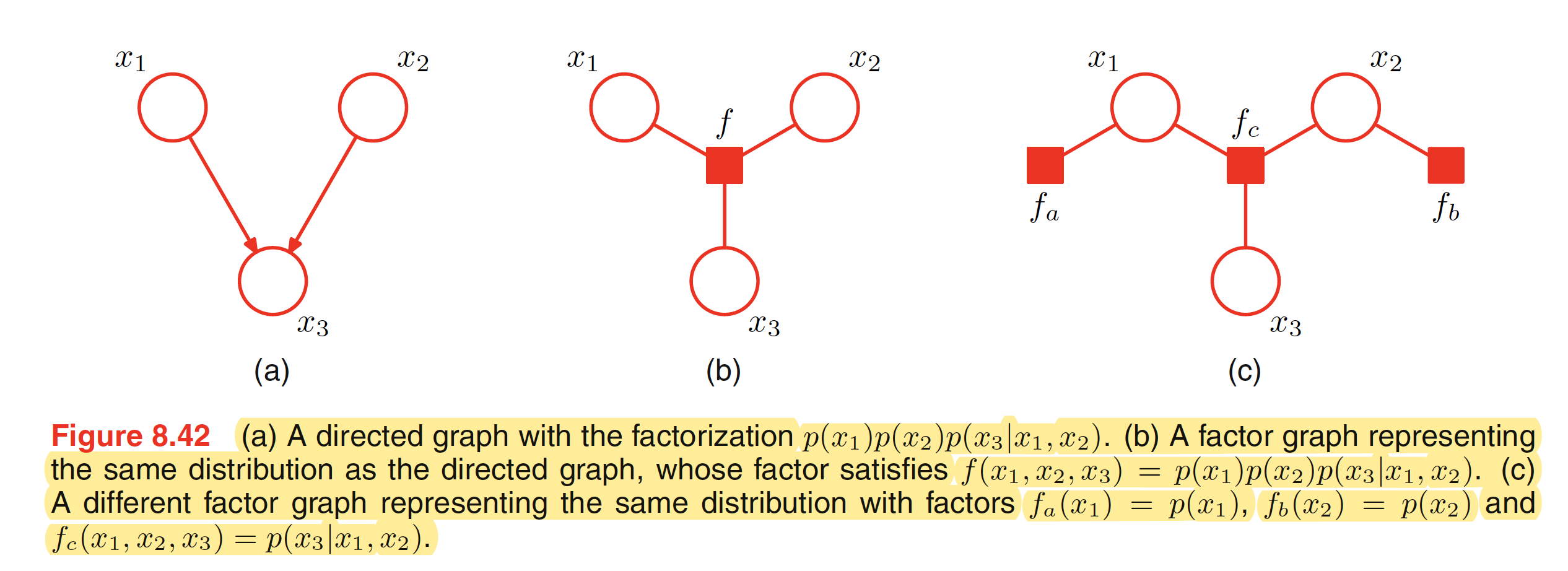
In a factor graph, there is a node (depicted by a circle) for every variable in the distribution. Additional nodes depicted by small squares for each factor $f_s(X_s)$ are also present. There are undirected links connecting each factor node to all the variable nodes on which that factor depends. For example, a joint distribution with its factor representation and corresponding factor graph is shown below.
$$\begin{align} p(X) = f_a(x_1,x_2)f_b(x_1,x_2)f_c(x_2,x_3)f_d(x_3) \end{align}$$
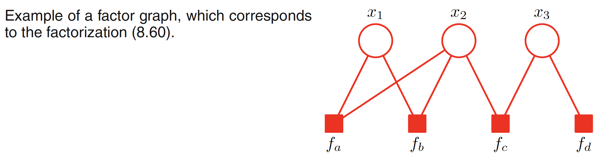
It should be noted that the first and the last two factors can be combined as a single potential as well but it is better to keep them explicit and hence conveying a more detailed information about the underlying factorization. Factor graphs are bipartite as they consist of two distinct kind of nodes and all links go between nodes of opposite type.
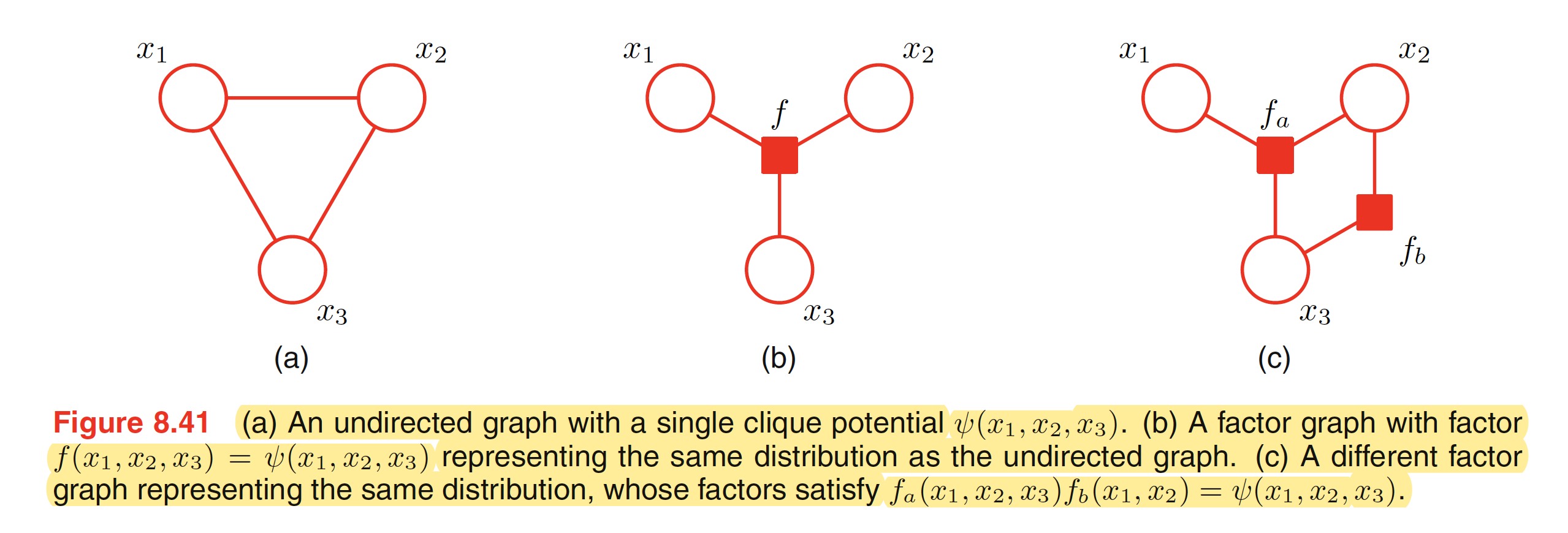
To convert an undirected graph to a factor graph, we need to create variable nodes corresponding to each node in the undirected graph. Apart from this, additional factor node corresponsing to each of the maximum clique is needed. There can be multiple factor graphs that correspond to the same undirected graph. One of the examples is shown below.
To convert a directed graph to a factor graph, we simply create variable nodes in the factor graph corresponding to the nodes of the directed graph, and then create factor nodes corresponding to the conditional distributions, and then finally add the appropriate links. Again, there can be multiple factor graphs all of which correspond to the same directed graph.