8.3 Markov Random Fields
A Markov random field, also known as a Markov network or an undirected graphical model has a set of nodes each of which corresponds to a variable or grpup of variables and the undirected links each of which connects a pair of nodes.
8.3.1 Conditional Independence Properties
In a directed graph, d-separataion can be used to check the conditional independence property. By removing the directed links from the graph, the assymetry between parent and child nodes is removed and hence the logic of d-separation can’t be applied directly.
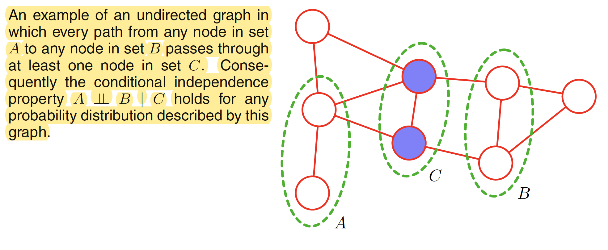
In an undirected graph, let $A,B,C$ are the three set of nodes which are considered for the conditional independence property $A \perp B | C$. To test whether this property is satisfied or not, we consider all possible paths that connects nodes in set $A$ to nodes in set $B$. If all such paths pass through one or more nodes in set $C$, then all such paths are blocked and hence the conditional independence property holds. If there at least exist one path which is not blocked, then the property does not hold. This means that there exists at least one distribution corresponding to the graph that do not satisfy the conditional independence relation. Following figure shows an example. As all the paths between $A$ and $B$ passes through nodes in $C$, the conditional independence property $A \perp B | C$ holds true.
An alternative way to view the conditional independence test is to imagine removing all nodes in set $C$ from the graph together with any links that connect to those nodes. We then ask if there exists a path that connects any node in $A$ to any node in $B$. If there are no such paths, then the conditional independence property must hold.
8.3.2 Factorizing Properties
The goal is to factorize an undirected graph based on the above conditional independence test. First of all for any two nodes $x_i$ and $x_j$ in an undirected graph, if they are not connected by a link then they are conditionally independent given all other nodes in the graph. This conditional independence property can be expressed as
$$\begin{align} p(x_i,x_j| X\setminus{x_i,x_j}) = p(x_i| X\setminus{x_i,x_j})p(x_j| X\setminus{x_i,x_j}) \end{align}$$
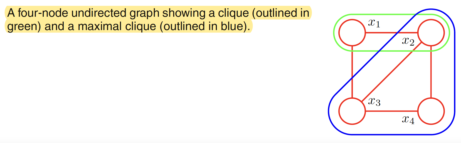
where $X\setminus{x_i,x_j}$ denotes set of all nodes apart from $x_i,x_j$. A clique is defined as a subset of the nodes in a graph such that there exists a link between all pairs of nodes is the subset. This means that the set of nodes in a clique is fully connected. A maximal clique is a clique such that it is not possible to include any other node from the graph in the set without it ceasing to be a clique. An example is shown below. The graph has two maximal cliques: ${x_1,x_2,x_3}, {x_2,x_3,x_4}$. Every two node pair apart from ${x_1,x_4}$ is a clique.
Let a clique be denoted by $C$ and the set of variables in it by $X_C$. Then the joint distribution is written as a product of potential functions $\Psi_C(X_C)$ over all the maximal cliques in the graph
$$\begin{align} p(X) = \frac{1}{Z}\prod_{C} \Psi_C(X_C) \end{align}$$
The quantity $Z$, called as the partition function is a normalization constant and is given as
$$\begin{align} Z = \sum_{X}\prod_{C} \Psi_C(X_C) \end{align}$$
This ensures that the distribution $p(X)$ is correctly normalized. By considering the potential function $\Psi_C(X_C) \geq 0$, we ensure that $p(X) \geq 0$. For the case of continuous variables, summation is replaced by integration in the above equation. The presence of this normalization coefficient is one of the major limitations of an undirected graph. However, for evaluation of a local conditional distribution, normalization coefficient is not needed as a local conditional distribution is ratio of two marginals and hence the normalization coefficoents cancel out.
Consider the set of all possible distributions defined over a fixed set of variables corresponding to the nodes of a particular undirected graph. Set $UI$ is a set of distributions which are consistent with the set of conditional independence statements interpreted from the graph. Set $UF$ be the set of such distributions which can be expressed as a factorization of the above form with respect to the maximal cliques of the graph. The Hammersley-Clifford theorem states that $UI$ and $UF$ are identical.
The potential functions can be represented as
$$\begin{align} \Psi_C(X_C) = exp {-E(X_C)} \end{align}$$
where $E(X_C)$ is called as the energy function and the exponential representation is called the Boltzmann distribution. The joint distribution is defined as the product of individual potentials and hence the total energy is obtained by adding the energies of each of the maximal cliques.
8.3.3. Illustration: Image De-noising
Let the observed noisy image be described by an array of binary pixel values $y_i \in {-1,+1}$, where the index $i=1,2,…,D$ runs over all the pixels. The origianl noise-free image is described by the binary pixel values $x_i \in {-1,+1}$ which is then flipped with some small probability, say $10%$. As the noise level is small, there will be strong correlation between $x_i$ and $y_i$. The neighbouring pixels $x_i$ and $x_j$ will also be strongly correlated. The undirected graph corresponding to this scenario is shown in the following figure.
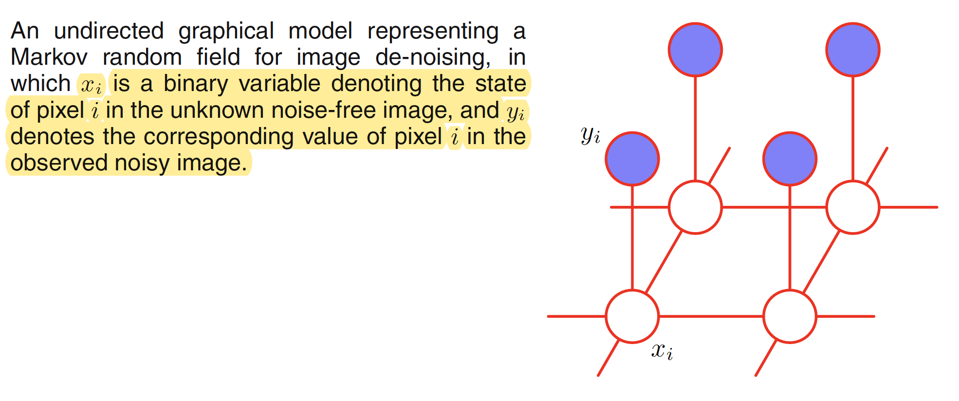
This graph has two type of cliques: ${x_i,y_i}$ and ${x_i,x_j}$. These cliques have an associated energy functions which express the correlation between these variables. The energy function for the clique associated with ${x_i,y_i}$ is chosen as $-\eta x_i y_i$ where $\eta$ is a positive constant. This gives higher energy to the graph if $x_i$ and $y_i$ are of opposite sign and lower energy if they are of the same sign. The energy function associated with ${x_i,x_j}$ is chosen as $-\beta x_i x_j$ where $\beta$ is a positive constant. This again has the affect of lower energy if the neighboring pixels are of the same sign. An extra term $hx_i$ for each pixel $i$ in the noise-free image can be added to the energy function. This term has an effect of biasing the model towards the pixel values that have one particular sign in preference to the other. The complete energy function of the model takes the form
$$\begin{align} E(X,Y) = h \sum_i x_i - \beta \sum_{{i,j}} x_ix_j - \eta \sum_i x_iy_i \end{align}$$
This defines a joint distribution over $X,Y$ given by
$$\begin{align} p(X,Y) = \frac{1}{Z} \exp {-E(X,Y)} \end{align}$$
The elements of noisy image $Y$ are fixed to the observed value, which implicitly defines a conditional distribution $p(X|Y)$ over noise-free images. For the purpose of image restoration, we need to find an image $X$ which has a high probability given the noisy image $Y$. This can be done using a simple iterative technique called as iterated conditional modes (ICM). The idea is to first assign the variables ${x_i}$, which can be done as $x_i = y_i$ for all $i$. Now a node $x_j$ is taken and total energy is evaluated for the two possible states $x_j = \pm 1$, keeping all the other variables fixed. $x_j$ is set to the state which has lower energy. This will either leave the probability unchanged (if $x_j$ is unchanged) or will increase it. The process is repeated until a suitable stopping criterian is met. The algorithm will converge to the local maxima which may not correspod to global maxima.
8.3.4 Relation to Directed Graphs
Let us try to derive the relation between a directed and an undirected graphical models. Consider first the problem of taking a model represented by a directed graph and convert it to an undirected one. Below figure shows a directed graph and its corresponding undirected representation.
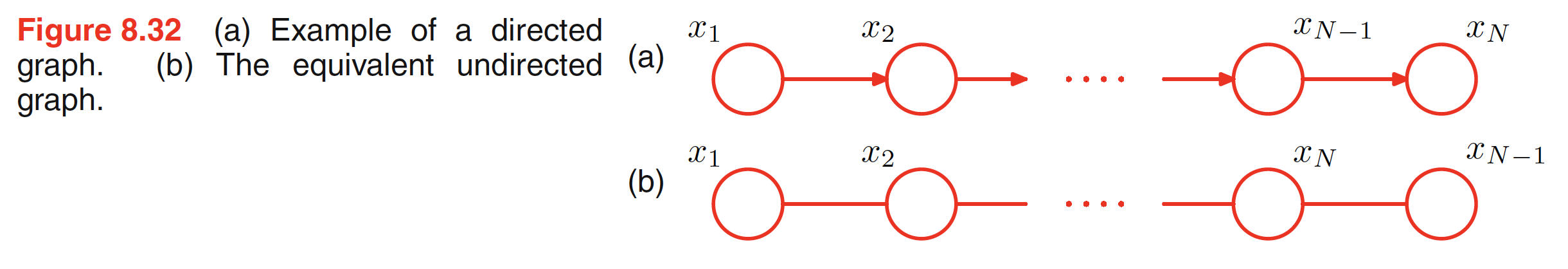
The joint distribution for the above connected graph is given as
$$\begin{align} p(X) = p(x_1)p(x_2|x_1)p(x_3|x_2)…p(x_N|x_{N-1}) \end{align}$$
The converted undirected graph representation is shown in the second grpah. In the undirected graph, the maximal cliques are the the pairs of neighbouring nodes. The joint distribution can then be given as the product of the potential functions over all the maximal cliques and takes the form
$$\begin{align} p(X) = \frac{1}{Z} \Psi_{1,2}(x_1,x_2) \Psi_{2,3}(x_2,x_3) … \Psi_{N-1,N}(x_{N-1},x_N) \end{align}$$
Comparing this with the joint distribution of the directed graph, we have
$$\begin{align} \Psi_{1,2}(x_1,x_2) = p(x_1)p(x_2|x_1) \end{align}$$
$$\begin{align} \Psi_{1,2}(x_2,x_3) = p(x_3|x_2) \end{align}$$
$$\begin{align} \Psi_{N-1,N}(x_{N-1},x_3) = p(x_N|x_{N-1}) \end{align}$$
The partition function $Z$ is given as $Z=1$.
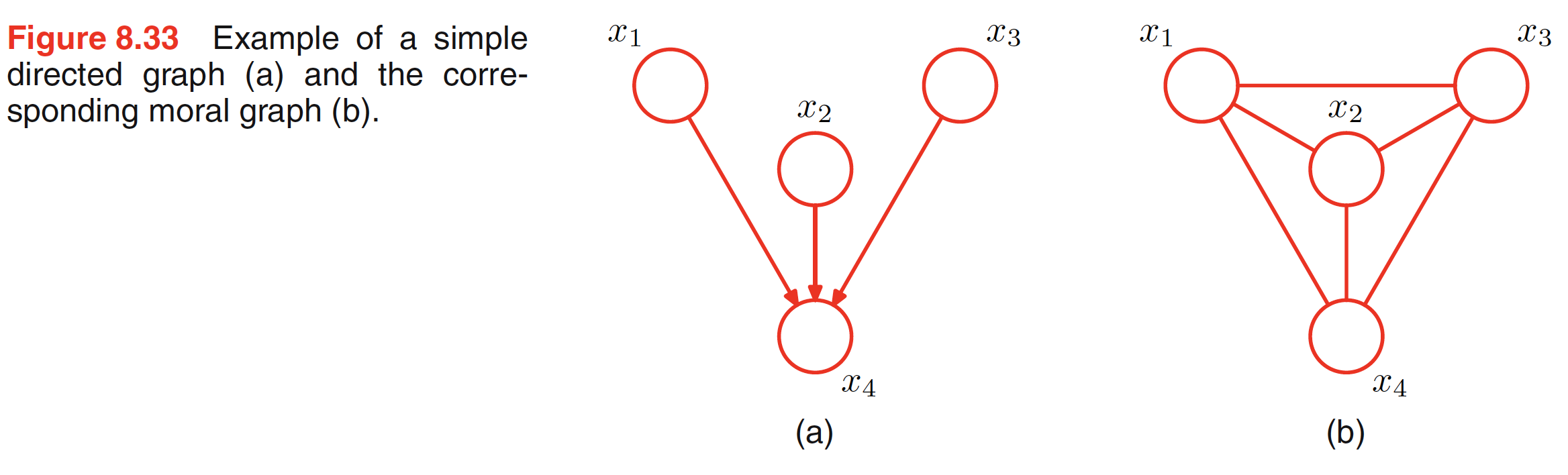
From the above example, it is clear that to convert a general directed graph to undirected graph, the clique potentials of the undirected graph are given by the conditional distributions of the directed graph. For this to be valid, we must ensure that the set of variables which appear in each of the conditional distributions is a member of at least one clique of the undirected graph. For nodes of the directed graph having one parent, this can be acheived simply by replacing the directed link with the undirected link. For the nodes which have more than one parent, this is not sufficient. For example, consider the below figure in which the node $x_4$ has three parents $x_1,x_2,x_3$. This means that in the correspodning undirected graph, the nodes $x_1,x_2,x_3,x_4$ should belong to the same clique, i.e. the parents need to be conncted or married. Hence, in the corresponding undirected graph parents are connected and arrows are dropped. This process of marrying the parents is called as moralization and the resulting undirected graph is called as moral graph. Hence, to convert any directed graph to undirected graph, we first additional undirected links between all pairs of parents for each node in the graph and then drop the arrows. Then we initialize all of the clique potentials of the moral graph to $1$. We then take each conditional distribution factor in the original directed graph and multiply it into one of the clique potentials.
In going from a directed to an undirected graph, we have to discard some of the conditional independence properties. We could always trivially convert any distribution over a directed graph into one over an undirected graph by simply using a fully connected undirected graph. A graph is said to be a D map (for dependency map) of a distribution if every conditional independence statement satisfied by the distribution is reflected in the graph. This means a completely disconnected graph (with no links) will be a trivial D map for any distribution.
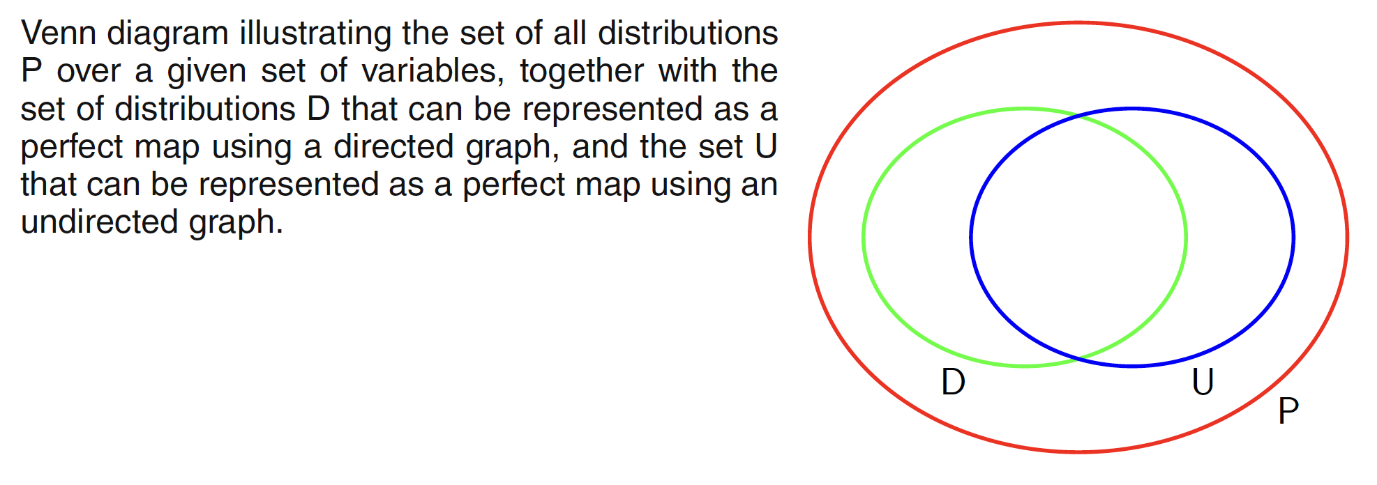
If every conditional independence statement implied by a graph is satisfied by a specific distribution, then the graph is said to be an I map (for independence map) of that distribution. Clearly a fully connected graph will be a trivial I map for any distribution. If every conditional independence property of the distribution is reflected in the graph, then the graph is said to be perfect map. A perfect map is therefore both an I map and a D map. Below figure shows how all the possible distributions over a given set of variables are spread across representation as a perfect map by directed and undirected graph.