8.2 Conditional Independence
Consider three variables $a,b,c$ and suppose that the conditional distribution of $a$ given $b$ and $c$ is such that it does not depend on value of $b$, i.e.
$$\begin{align} p(a|b,c) = p(a|c) \end{align}$$
We say that $a$ is conditionally independent of $b$ given $c$. This can be expressed in a different way if we consider the joint distribution of $a$ and $b$ conditioned on $c$, which can be written as
$$\begin{align} p(a,b|c) = p(a|b,c)p(b|c) = p(a|c)p(b|c) \end{align}$$
Hence, conditioned on $c$, the joint distribution of $a$ and $b$ factorizes into the product of marginal distribution of $a$ and the marginal distribution of $b$ (both conditioned on $c$). This means that variables $a$ and $b$ are statistically independent, given $c$. This can be denoted as
$$\begin{align} a \perp b | c \end{align}$$
which means that $a$ is conditionally independent of $b$ given $c$. In a graphical model, the conditional independence property can be directly read from the graph without any analytical manipulations.
8.2.1 Three Example Graphs
The conditional independence properties of directed graphs can be considered using three simple examples each having juts three node. The first of the three examples is shown below.
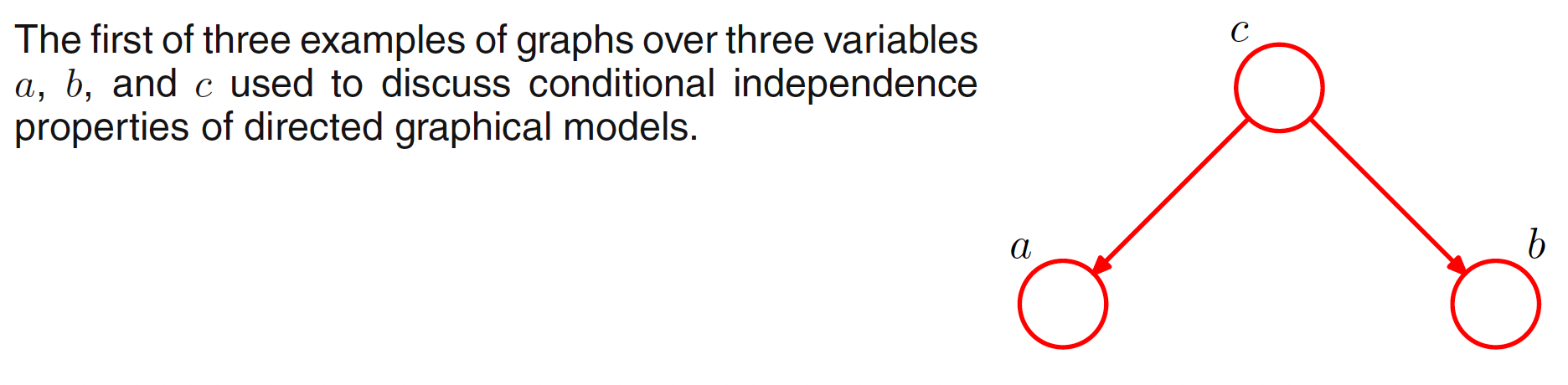
The joint distribution corresponding to the above graph is given as
$$\begin{align} p(a,b,c) = p(a|c)p(b|c)p(c) \end{align}$$
If none of the variables are observed, then we can investigate whether $a$ and $b$ are independent by marginalizing both sides of above equation with respect to $c$ as
$$\begin{align} p(a,b) = \sum_{c}p(a|c)p(b|c)p(c) \end{align}$$
In general, this doesn’t factorize into $p(a)p(b)$ and we can say that
$$\begin{align} a \text{ not}\perp b | \emptyset \end{align}$$
where $\emptyset$ denotes the empty set and $\text{ not}\perp$ means that the conditional independence property does not hold. If we observe the variable $c$, i.e. we condition on the variable $c$, the above graph is modified as
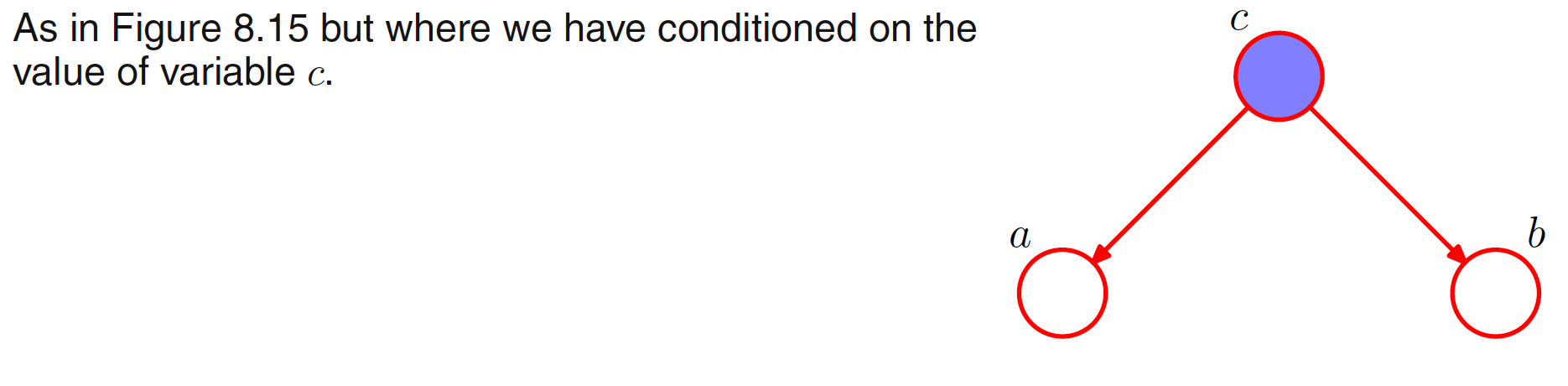
The conditional distribution of $a$ and $b$ given $c$ can be written as
$$\begin{align} p(a,b|c) = \frac{p(a,b,c)}{p(c)} = p(a|c)p(b|c) \end{align}$$
and hence we obtain the conditional independence property
$$\begin{align} a \perp b | c \end{align}$$
A simple graphical explanation of this result can be given by considering the path from node $a$ to node $b$ via node $c$. The node $c$ is said to be tail-to-tail with respect to this path because the node is connected to the tails of the two arrows and the presence of such a path connecting nodes $a$ and $b$ cause these nodes to be dependent. If node $c$ is observed, this path is blocked and causes node $a$ and $b$ to become (conditionally) independent.
The second example is shown below.
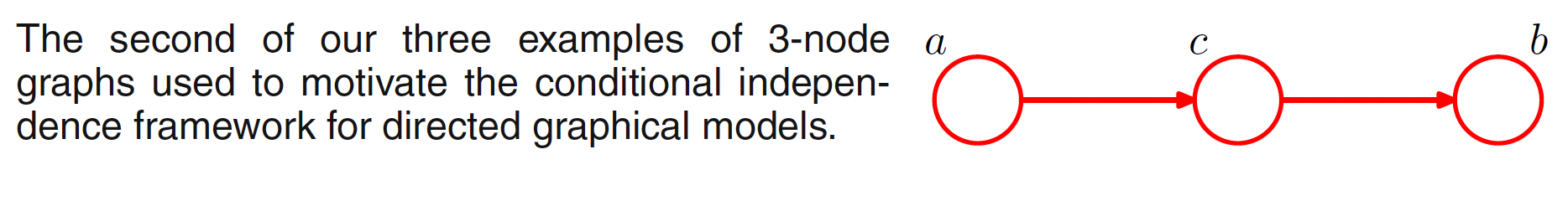
The joint distribution corresponding to this graph is given as
$$\begin{align} p(a,b,c) = p(a)p(c|a)p(b|c) \end{align}$$
For the case, when none of the variables are observed, the joint distribution of $a$ and $b$ can be obtained by marginalizing over $c$ and is given as
$$\begin{align} p(a,b) = p(a)\sum_{c}p(c|a)p(b|c) = p(a)p(b|a) \end{align}$$
which in general does not factorize into $p(a)p(b)$ and hence
$$\begin{align} a \text{ not}\perp b | \emptyset \end{align}$$
Now suppose, node $c$ is observed, i.e. we condition on node $c$, then we have
$$\begin{align} p(a,b|c) = \frac{p(a,b,c)}{p(c)} = \frac{p(a)p(c|a)p(b|c)}{p(c)} = p(a|c)p(b|c) \end{align}$$
and hence we obtain the conditional independence property
$$\begin{align} a \perp b | c \end{align}$$
This result can be interpretted graphically. Node $c$ is said to be head-to-tail with respect to the path from node $a$ to node $b$. Such a path connects node $a$ and node $b$ and renders them dependent. If node $c$ is observed, this path is blocked and hence we obtain the conditional independence property.
The third example is shown in the following figure.
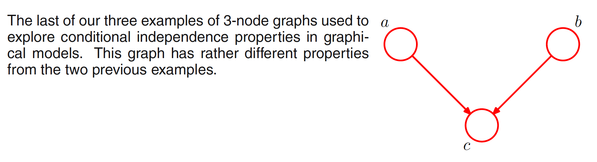
The joint distribution corresponding to this graph can be written as
$$\begin{align} p(a,b,c) = p(a)p(b)p(c|a,b) \end{align}$$
When none of the variables are observed, marginalizing both sides over $c$, we have
$$\begin{align} p(a,b) = \sum_{c}p(a)p(b)p(c|a,b) = p(a)p(b) \end{align}$$
This means that $a$ and $b$ are idependent when no variables are observed, i.e.
$$\begin{align} a \perp b | \emptyset \end{align}$$
Now suppose that $c$ is observed. The conditional distribution of $a$ and $b$ is then given as
$$\begin{align} p(a,b|c) = \frac{p(a,b,c)}{p(c)} = \frac{p(a)p(b)p(c|a,b)}{p(c)} \neq p(a)p(b) \end{align}$$
and hence, we have
$$\begin{align} a \text{ not}\perp b | c \end{align}$$
Graphically, we say that node $c$ is head-to-head with respect to the path from $a$ to $b$ as it connects the head of the two arrows. When node $c$ is unobserved, it blocks the path and hence variables $a$ and $b$ are independent. Conditioning on $c$ unblocks the path and that renders $a$ and $b$ dependent.
In summary, a tail-to-tail node or a head-to-tail node leaves a path unblocked (and hence dependency) until it is observed in which case the path is blocked (and hence independency). By contrast, a head-to-head node blocks a path if $v \notin C$ and no descendent of $v$ is in $C$. We say that node $y$ is a descendant of node $x$ if there is a path from $x$ to $y$ in which each step of the path follows the direction of the arrow.
8.2.2 D-Separation
Consider a general directed graph in which $A,B,C$ are arbitrary nonintersecting sets of nodes. We want to ascertain whether a particular conditional independence statement $A \perp B | C$ is implied by a directed acyclic grpah or not. The d-sepafation theorem states that if $A$ and $B$ are d-separated by $C$ then $A \perp B | C$. $A$ and $B$ are d-separated by $C$ if all the paths from a vertex of $A$ to a vertex of $B$ are blocked with respect to $C$ [https://youtu.be/aA-gTNxy1rw].
To find the d-separation, we cosider the all possible paths from any node in $A$ to any node in $B$. Any such path is said to be blocked if it includes a node such that it either
-
the arrows on the path meet either head-to-tail or tail-to-tail (i.e. a tail is involved) at the node and the node is observed, and the node is in the set $C$, or
-
the arrows meet head-to-head at the node, and neither the node, nor any of its descendants, is in the set $C$.
If all paths are blocked, then $A$ is said to be d-separated from $B$ by $C$, and the joint distribution over all of the variables in the graph will satisfy $A \perp B | C$. The concept of d-separation is shown in following figure.
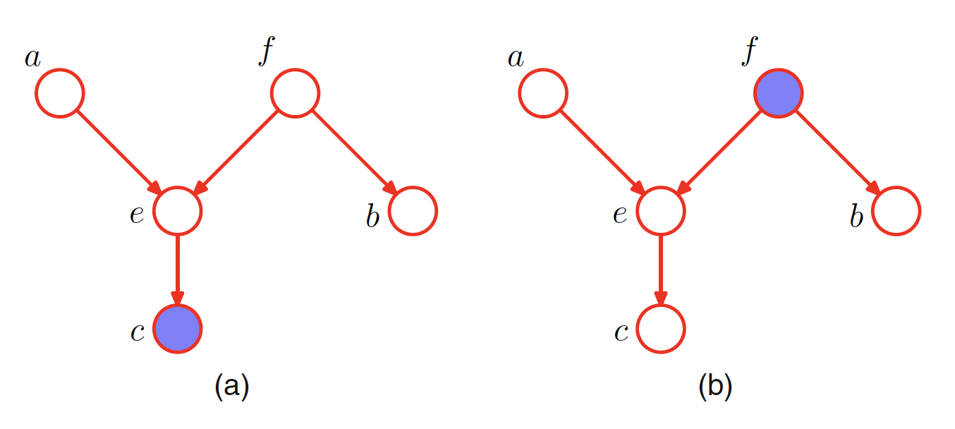
In the graph $(a)$, the path from $a$ to $b$ via $f$ is tail-to-tail and the node $f$ is not observed and hence is not blocked. The path from $a$ to $b$ via $e$ is head-to-head and it has a descendnt $c$ which is in the conditioning set and hence the path is not blocked. This means that the conditional independence statement $a \perp b | c$ does not follow from the graph.
In the graph $(b)$, the path from $a$ to $b$ via node $f$ is tail-to-tail and $f$ is observed and hence the path is blocked. This means that the conditional independence property $a \perp b | f$ is satisfied by any distribution which factorizes according to this graph.
Another example of conditional independence and d-separataion is provided by the concept of i.i.d. (independent identically distributed) data. Consider the problem of finding the posterior distribution for the mean of univariate Gaussian. The distribution can be represnted by the following graph where the joint distribution is defined by a prior $p(\mu)$ and $p(x_n|\mu)$ where $n=1,2,…,N$. We observe $D={x_1, x_2,…,x_N}$ and our goal is to infer $\mu$.
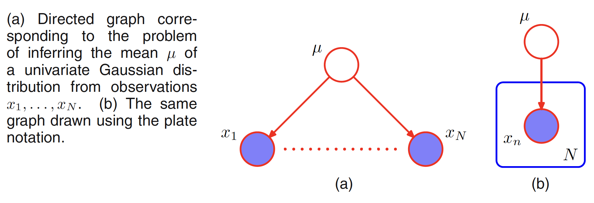
When conditioned on $\mu$, there is a unique path from $x_i$ to any other $x_{j \neq i}$ via $\mu$. This path is tail-to-tail and node $\mu$ being observed, the path is blocked. Hence, we have
$$\begin{align} p(D|\mu) = \prod_{n=1}^{N} p(x_n|\mu) \end{align}$$
While integrating over $\mu$, the the condition of independence is no longer satisfied as $\mu$ is not observed now and hence
$$\begin{align} p(D) = \int_{0}^{\infty}p(D|\mu)p(\mu)d\mu \neq \prod_{n=1}^{N} p(x_n) \end{align}$$
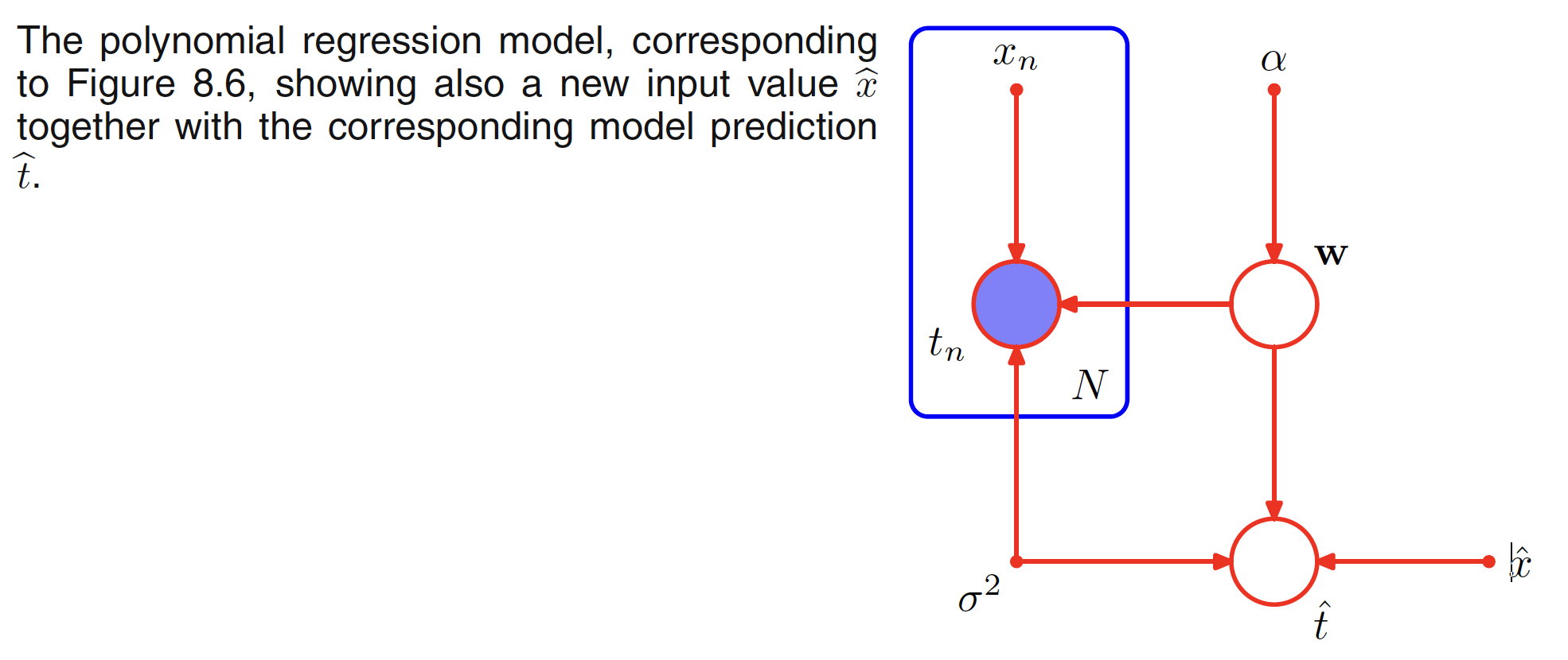
Another use of d-separation is shown in the below graph for the Bayesain polynomial regression. The stochastic nodes in the graph are ${t_n}, w, \hat{t}$. For the path from $\hat{t}$ to any node in ${t_n}$, node $w$ is tail-to-tail. When $w$ is observed, the path is blocked and hence $\hat{t} \perp t_n | w$. This means that conditioned on the polynomial coefficients $w$, the predictive distribution for $\hat{t}$ is independent of the training data ${t_1, t_2, …, t_N}$. We can hence use the training data to derermine the posterior distribution for $w$. The training data then can be discarded and the posterior distribution of $w$ can be used to make predictions $\hat{t}$ for the new input $\hat{x}$.
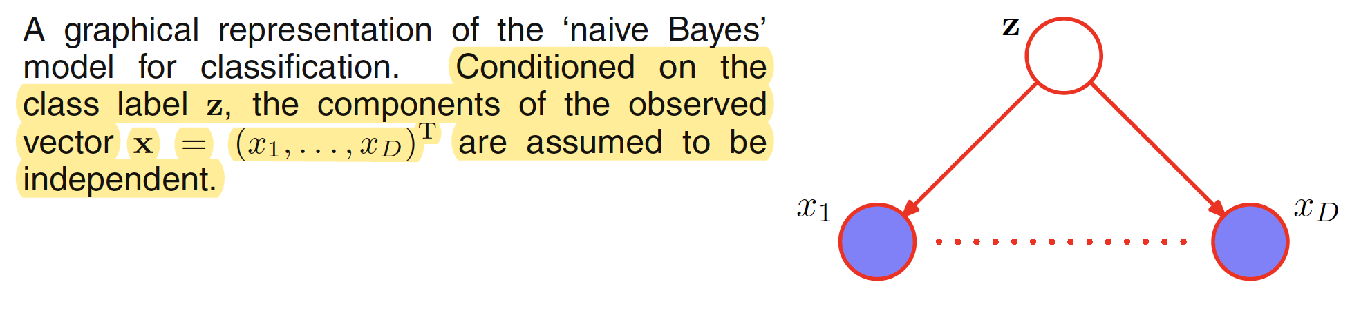
The conditional independence assumption can be used to simplify the model structure for a naive Bayes model. Let the observed input variable $x$ be a D-dimensional vector $x = (x_1,x_2,…,x_D)^T$ and we wish to assign $x$ to one of the $K$ classes. Using $1-of-K$ encoding, these classes can be represented by a K-dimensional binary vector $z$. A multinomial prior ovee the class labels can be defined as $p(z|\mu)$ where the $k^{th}$ component $\mu_k$ of $\mu$ is the probability of class $C_k$. The key assumption of the naive Bayes model is: conditioned on $z$, the distributions of the input variables $x_1,x_2,…,x_D$ are independent. The graphical representation of this model is shown below. The path between $x_i$ to $x_j$ where $j \neq i$ is tail-to-tail at the node $z$ and $z$ being observed blocks this path. This makes $x_i$ and $x_j$ connditionally independent given $z$. If we marginalize out $z$ (i.e. $z$ is unobserved), the path is no longer blocked and hence in general the marginal density $p(x)$ will not factorize with respect to the components of $x$.
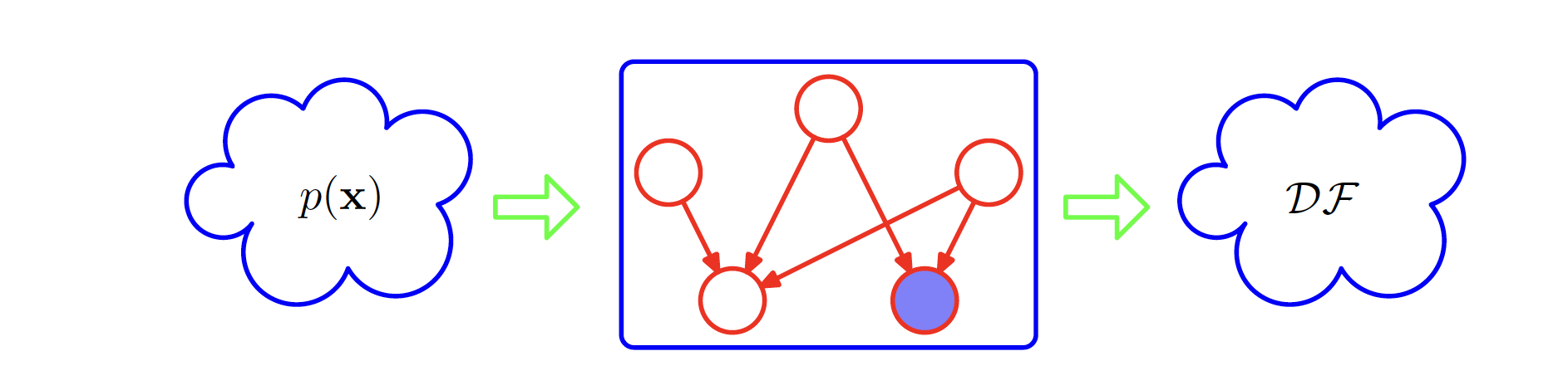
Directed Graphs can be thought of a filter. For a particular joint probability distribution $p(x)$ over the variables $x$ corresponding to the nodes of the graph, the filter will allow this distribution to pass through if and only if it can be expressed in terms of the factorization implied by the graph. If all possible distributions $p(x)$ are presented to the filter, then the subset of distributions that are passed by the filter will be denoted as $DF$, for directed factorization. This is shown in the following figure. The two extremes of the graps can be a fully connected graph which exhibits no conditional independence property and which can represent any possible joint distributio over the given variables. The other extreme is a fully disconnected graph which corresponds to joint distribution which factorise into the product of the marginal distribution of the nodes in the graph.
A Markov blanket or Markov boundary of a node $x_i$ is the minimal set of nodes that isolates $x_i$ from the rest of the graph. It is i,lustrated in the following figure. The conditional distribution of node $x_i$ conditioned on the remaining nodes in the graph depends only on the variables in the Markov blanket.