Probabilistic models can also be analyzed using diagrammatic representations of probability distributions, called probabilistic graphical models. A graph comprises nodes (also called vertices) connected by links (also known as edges or arcs). Each node represents a random variable (or group of random variables), and the links express probabilistic relationships between these variables. Graph then captures the way in which the joint distribution over all of the random variables can be decomposed into a product of factors each depending only on a subset of the variables.
Bayesian networks, also known as directed graphical models, are the graphs in which links of the graphs have a particular directionality indicated by arrows. Markov random fields, also known as undirected graphical models, are the graphical models in which the links do not carry arrows and have no directional significance. Directed graphs are useful for expressing causal relationships between random variables, whereas undirected graphs are better suited to expressing soft constraints between random variables.
8.1 Bayesian Networks
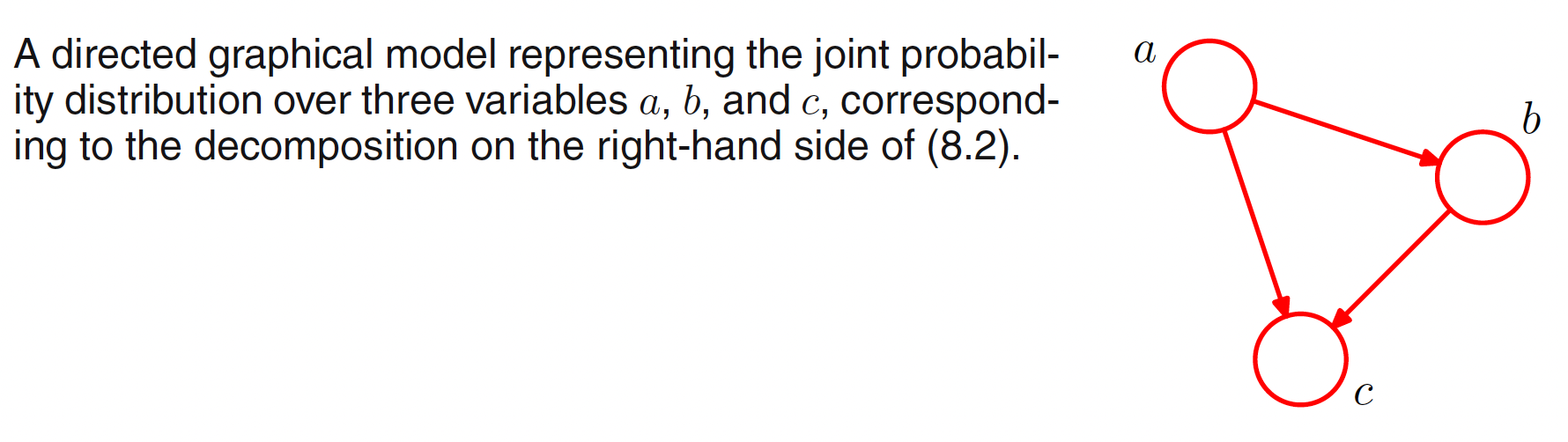
A joint distribution $p(a,b,c)$ over three variables $a,b,c$ can be represented as
$$\begin{align} p(a,b,c) = p(c|a,b)p(b|a)p(a) \end{align}$$
Above decompositon holds for any choice of joint distribution. To represent this as graphical representation, we introduce a node for each of the random variables $a, b, c$ and associate each node with the corresponding conditional distribution on the right-hand side. For each conditional distribution we add directed links (arrows) to the graph from the nodes corresponding to the variables on which the distribution is conditioned. For factor $p(c|a,b)$ there will be links from nodes $a,b$ to node $c$ and whereas for factor $p(a)$ there will be no incoming links. If there is a link going from node $a$ to node $b$, then we say that node $a$ is the parent of node $b$, and node $b$ is the child of node $a$. The graphical representation of above decomposition of the joint distribution is shown below. It should be noted that the graphical representation depends on how we decompose the joint distribution.
The joint distribution over $K$ variables can be similarly decomposed as
$$\begin{align} p(x_1,x_2,…,x_K) = p(x_K|x_1,…,x_{K-1})…p(x_2|x_1)p(x_1) \end{align}$$
In the graphical representation of above decomposition, each node has incoming links from all lower numbered nodes. The graph will be fully connected as there is a link between every pair of nodes. For a completely general joint distribution, the representation of the decomposition will be fully connected graphs. But it is the absence of links in the graph that conveys interesting information about the properties of the class of distributions that the graph represents. For example, below graph is not fully connected.
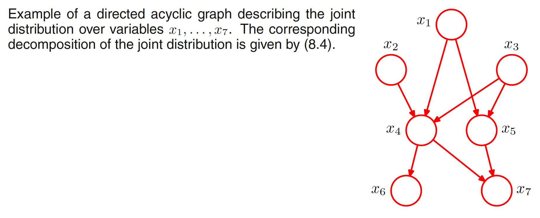
For the above graph, the representation of the joint distribution as the product of the set of conditional distributions (one for each node) is:
$$\begin{align} p(x_1)p(x_2)p(x_3)p(x_4|x_1,x_2,x_3)p(x_5|x_1,x_3)p(x_6|x_4)p(x_7|x_4,x_5) \end{align}$$
Hence, the joint distribution defined by a graph is given by the product, over all of the nodes of the graph, of a conditional distribution for each node conditioned on the variables corresponding to the parents of that node in the graph. For a graph with $K$ nodes, the joint distribution is given as
$$\begin{align} p(X) = \prod_{k=1}^{K}p(x_k|pa_k) \end{align}$$
where $pa_k$ denotes the set of parents of $x_k$ and $X={x_1,x_2,…,x_k}$. This equation represents the fatcorization property of the joint distribution for a directed graphical model.
The directed graphs that we are considering are subject to an important restriction namely that there must be no directed cycles, in other words there are no closed paths within the graph such that we can move from node to node along links following the direction of the arrows and end up back at the starting node. Such graphs are also called directed acyclic graphs, or DAGs. This is equivalent to the statement that there exists an ordering of the nodes such that there are no links that go from any node to any lower numbered node.
8.1.1 Example: Polynomial regression
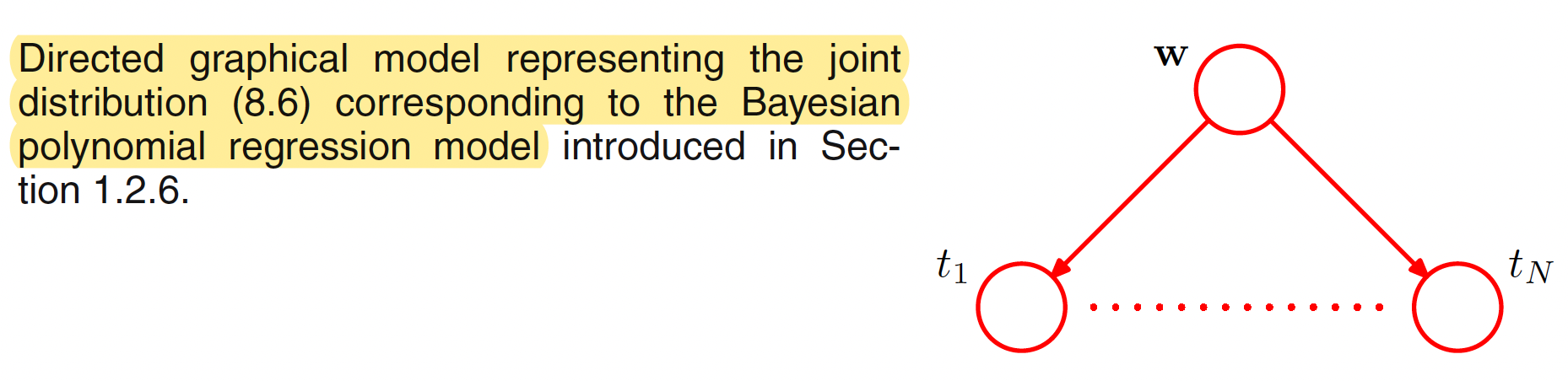
In a Bayesian Polynomial Regression, the vector of polynomial coefficients $W$ and and the observed data $t=(t_1,t_2,…,t_N)^T$ are the random variables. Apart from this, the other model parameters are the input $X=(x_1,x_2,…,x_N)^T$, the noise variance $\sigma^2$ and the hyeperparameter $\alpha$ representing the precison of the Gaussian prior over $W$. Focusing on the random variables, the joint distribution is given as
$$\begin{align} p(t, W) = p(W) \prod_{n=1}^{N}p(t_n|W) \end{align}$$
Its graphical representation is shown below.
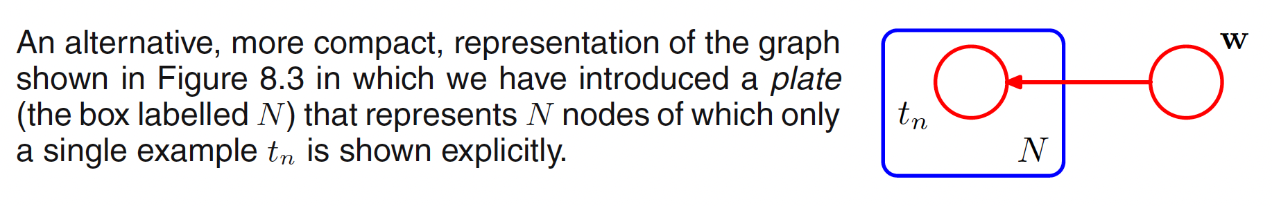
Above notation can be represented in a compact way by drawing a single representative node $t_n$ and then surround it with a box, called as plate, labelled with $N$ indicating that there are $N$ nodes of this kind. This representation is shown below.
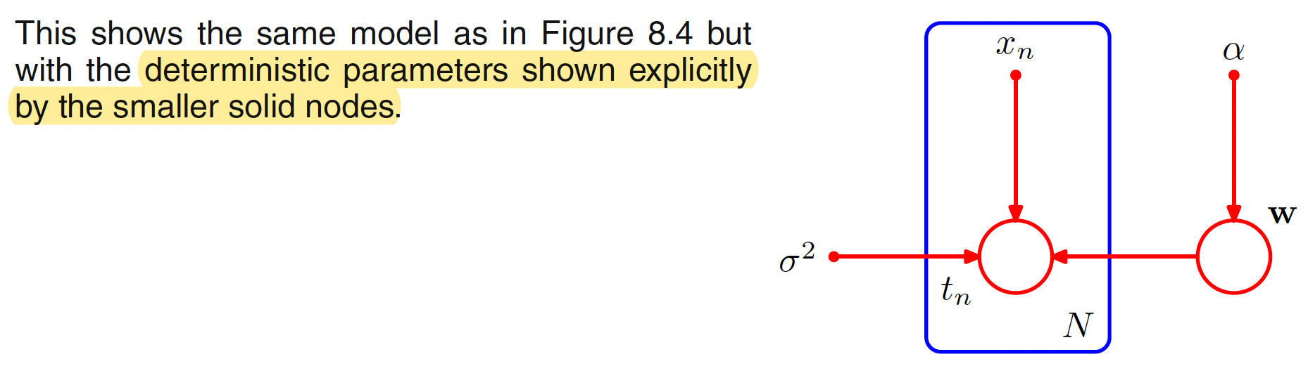
Making the parameters of the model and its stochastic variable explicit, the updated joint distribution is given as
$$\begin{align} p(t, W|X,\alpha,\sigma^2) = p(W|\alpha) \prod_{n=1}^{N}p(t_n|W,x_n,\sigma^2) \end{align}$$
Taking a notation that the random variables will be denoted by open circles and the deterministic parameters will be denoted by smaller solid circles, the graphical representation of above joint distribution is shown below.
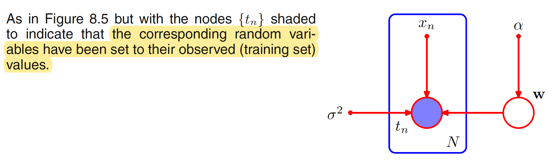
While applying the graphical model to a problem in machine learning, some of the random variables can be set to a specified observed values. For example, the varaibles $t=(t_1,t_2,…,t_N)^T$ from the training set in the case of polynomial curve fitting. These observed random variables can be denoted by shading the corresponding nodes. The graphical representation when ${t_n}$ is observed for the above joint distribution is shown below. The value of $W$ is not observed and is called as latent or hidden variable.
Using Bayes’ theorem, the posterior distribution of the coefficients $W$ is given as
$$\begin{align} p(W|t) = p(W) \prod_{n=1}^{N}p(t_n|W) \end{align}$$
where the deterministic parameters have been omitted to keep the notation uncluttered.
8.1.2 Generative Models
There are many situations in which we wish to draw samples from a given probability distribution. Consider a joint distribution $p(x_1,x_2,…,x_K)$ over $K$ variables that factorizes according to the following equation corresponding to a directed acyclic graph.
$$\begin{align} p(X) = \prod_{k=1}^{K}p(x_k|pa_k) \end{align}$$
where $pa_k$ denotes the set of parents of $x_k$. Without any loss of generalization, we can assume that the variables have been ordered such that there are no links from any node to any lower numbered node, i.e. each child has a higher number than any of its parents. Our goal is to draw a sample $\hat{x_1}, \hat{x_2}, …, \hat{x_K}$ from the joint distribution.
To do this, we start with the lowest-numbered node and draw a sample from the joint distribution $p(x_1)$ which we call $\hat{x_1}$. We then work through each of the nodes in order, so that for node $x_n$ we draw a sample from the conditional distribution $p(x_n|pa_n)$ in which the parent variables have been set to their sampled values. At each stage, these parent values will always be available because they correspond to lower numbered nodes that have already been sampled. Once we have sampled from the final variable $x_K$, we will have achieved our objective of obtaining a sample from the joint distribution. To obtain a sample from some marginal distribution corresponding to a subset of the variables, we simply take the sampled values for the required nodes and ignore the sampled values for the remaining nodes.
8.1.3 Discrete Variables
The probability distribution $p(x|\mu)$ for a single discrete varaible $x$ having $K$ possible states is given by
$$\begin{align} p(x|\mu) = \prod_{k=1}^{K} \mu_k^{x_k} \end{align}$$
and is governed by the parameters $\mu = (\mu_1, \mu_2, …, \mu_K)^T$. As we have a constraint $\sum_k \mu_k = 1$, only $K-1$ values for $\mu_k$ need to be specified in order to define ths distribution.
For the case of two discrete variables $x_1,x_2$, each of which has $K$ states, the probability of observing both $x_{1k} = 1$ and $x_{2l} = 1$ is given by the parameter $\mu_{kl}$. The joint distribution can then be written as
$$\begin{align} p(x_1, x_2|\mu) = \prod_{k=1}^{K}\prod_{l=1}^{K} \mu_{kl}^{x_{1k}x_{2l}} \end{align}$$
where the parametere $\mu_{kl}$ is subjected to the constraint $\sum_k\sum_l\mu_{kl} = 1$. This distribution is governed by $K^2-1$ parameters. For an arbitrary joint distribution over $M$ variables, total number of parameters needed is given as $K^M-1$ and hence grows exponentially with the number of variables $M$.
The joint distribution $p(x_1,x_2)$ can be factored as $p(x_2|x_2)p(x_1)$, which corresponds to a two-node graph with a link going from the node $x_1$ to the node $x_2$. The marginal distribution $p(x_1)$ is governed by $K-1$ parameters. The conditional distribution $p(x_2|x_1)$ requires the specification of $K-1$ parameters for each of the $K$ possible values of $x_1$. The total number of parameters that must be specified in the joint distribution is therefore $(K-1) + K(K-1) = K^2-1$. When $x_1$ and $x_2$ are independent, the total number of parameters would be $2(K-1)$. Hence, for a distribution of $M$ independent discrete variables, each having $K$ states, the total number of parameters would be $M(K-1)$, which grows linearlly with the number of variables.
In general, if we have $M$ discrete variables $x_1,x_2,…,x_M$, we can model the joint distribution using a directed graph with one variable corresponding to each node. If the graph is fully connected, we have a completely general distribution having $K^M-1$ parameters. If there are no links, the total number of prameters is $M(K-1)$. Graphs having intermediate levels of connectivity allow for more general distributions. For example, consider the chain of nodes shown in below figure.
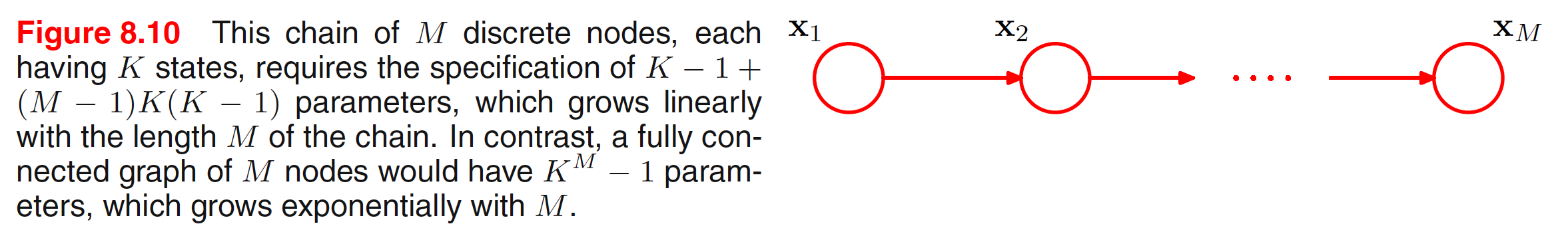
In the above connected graph, the marginal distribution $p(x_1)$ requires $K-1$ parameters. Each of the $M-1$ conditional distributions $p(x_i|x_{i-1})$ for $i=2,3,…,M$ requires $K(K-1)$ parameters. This gives a total parameter count of $K-1+(M-1)K(K-1)$. The number of parameters is quadratic in $K$ and which grows linearly with the length $M$ of the chain.
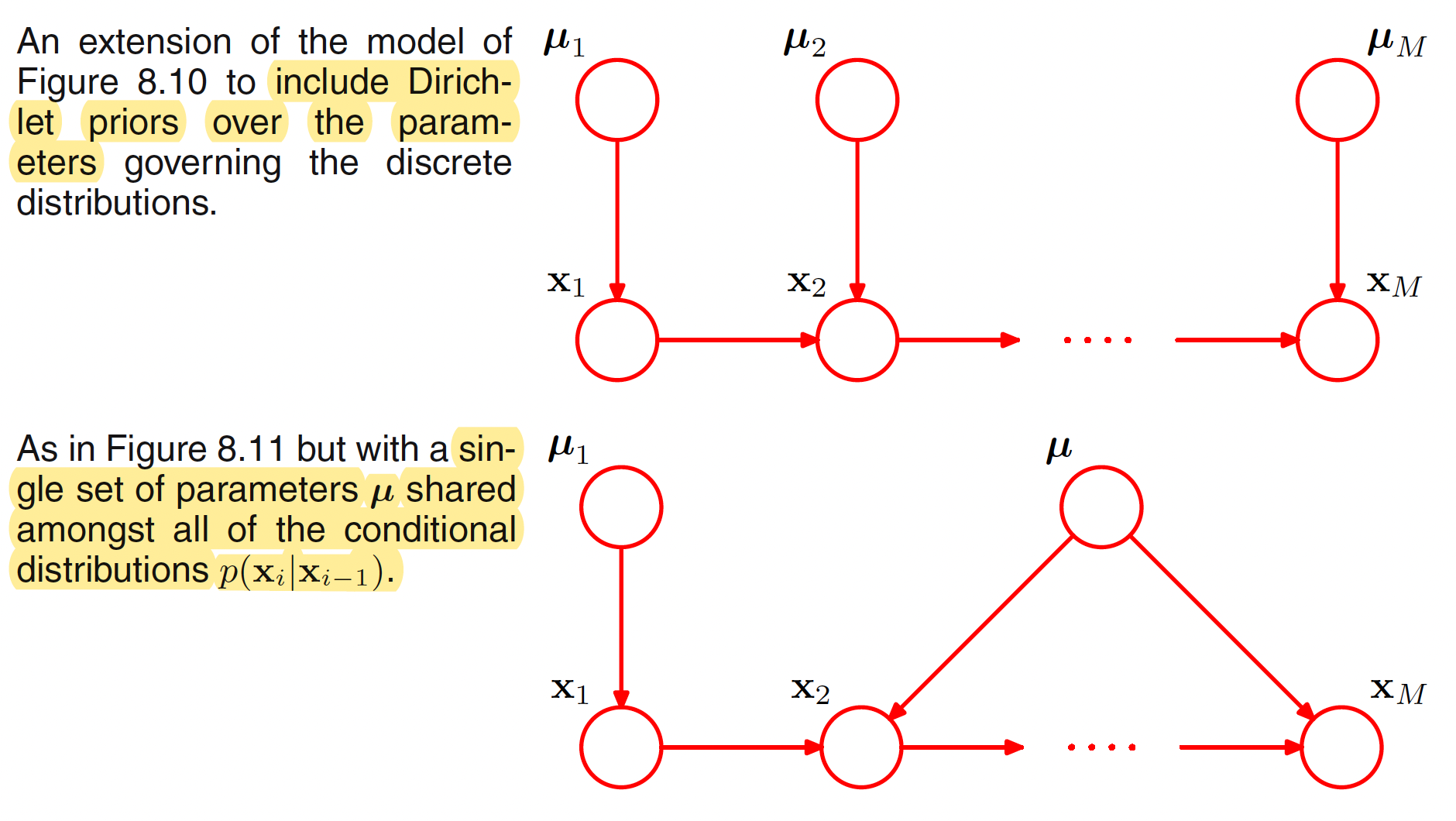
Another way to reduce the number of independent parameters in a model is by sharing of parameters. For example, in the above graphical model, all the conditional distributions $p(x_i|x_{i-1})$ for $i=2,3,…,M$ can be governed by the same set of $K(K-1)$ parameters. Together with the $K-1$ parameters for $x_1$, a total of $K-1+K(K-1) = K^2-1$ prameters are needed to define the joint distribution.
A graphical model over discrete variables can be turned into a Bayesian model by introducing priors (Dirichlet priors) to the parameters. Each node than has an additional parent representing the prior distribution over the parameters associated with the corresponding discrete node. This is illustrated in the following figure.
8.1.4 Linear-Gaussian Models
Consider an arbitrary directed acyclic graph over $D$ variables in which node $i$ represents a single continuous random variable $x_i$ having a Gaussian distribution. Then, we have
$$\begin{align} p(x_i|pa_i) = N\bigg(x_i \bigg| \sum_{j \in pa_i} w_{ij}x_j + b_i, v_i\bigg) \end{align}$$
where $w_{ij}$ and $b_i$ are the parameters governing the mean and $v_i$ is the variance of the conditional distribution for $x_i$. The joint distribution is then given as the product of these conditionals over all nodes in the graph and hence takes the form
$$\begin{align} p(x) = \prod_{i=1}^{D}p(x_i|pa_i) \end{align}$$
Taking logarithm, we have
$$\begin{align} \ln p(x) = \sum_{i=1}^{D}\ln p(x_i|pa_i) \end{align}$$
As we have
$$\begin{align} p(x_i|pa_i) = N\bigg(x_i \bigg| \sum_{j \in pa_i} w_{ij}x_j + b_i, v_i\bigg) = \frac{1}{\sqrt{2\pi v_i}}\exp {\bigg[\frac{-1}{2v_i} \bigg(x_i - \sum_{j \in pa_i} w_{ij}x_j - b_i \bigg)^2\bigg]} \end{align}$$
Hence,
$$\begin{align} \ln p(x) = -\sum_{i=1}^{D} \frac{1}{2v_i} \bigg(x_i - \sum_{j \in pa_i} w_{ij}x_j - b_i \bigg)^2 + const \end{align}$$
where $const$ denotes terms indendent of $x_is$. The logarithm of the joint distribution is quadratic in $x$ and hence the joint distribution $p(x)$ is a multivariate Gaussian.