7.1.2 Relation to Logistic Regression
For nonseparable case of SVM, for the data points that are on the correct side of margin, we have $\xi_n=0$ and hence $t_ny_n \geq 1$. For the remaining points, we have $\xi_n = 1 - t_ny_n$. The below objective function can then be written as
$$\begin{align} \frac{1}{2}||W||^2 + C\sum_{n=1}^{N}\xi_n = \lambda||W||^2 + \sum_{n=1}^{N}E_{SV}(t_ny_n) \end{align}$$
where $\lambda = (2C)^{-1}$ and $E_{SV}(.)$ is the hinge error function defined as
$$\begin{align} E_{SV}(t_ny_n) = [1-t_ny_n]_{+} \end{align}$$
where $[.]{+}$ denotes the positive part. This means that $E{SV}(z) = [1-z]{+} = 0$ when $z \geq 1$ and $E{SV}(z) = [1-z]_{+} = 1-z$ when $z < 1$. The plot of hinge error function is shown below.
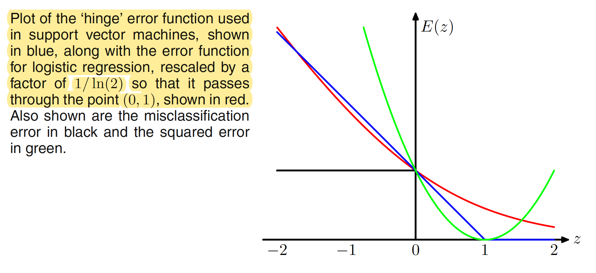
The plot of the hinge error function can be viewed as the approximation for the scaled misclassification error function used in logistic regression.
In the logistic regression model we worked with the target variable $t \in {0,1}$. To compare with SVM, we have to reformulate the logistic regression model to accomodate $t \in {-1,1}$. In a logistic regression model, we have $p(t=1|y) = \sigma(y)$. Hence, $p(t=-1|y) = 1 - p(t=1|y) = 1 - \sigma(y) = \sigma(-y)$ (from the property of logistic sigmoid function). We can say that
$$\begin{align} p(t|y) = \sigma(yt) = \frac{1}{1+\exp{(-yt)}} \end{align}$$
An error function can then be generated by taking the negative logarithm of the likelihood $p(t|y)$ and adding a quadratic regularizer as
$$\begin{align} -\ln p(t|y) = \sum_{n=1}^{N}E_{LR}(y_nt_n) + \lambda ||W||^2 \end{align}$$
where
$$\begin{align} E_{LR}(y_nt_n) = \ln (1 + \exp (-y_nt_n)) \end{align}$$
The rescaled version of this error function is plotted in red in the above figure and is quite similar to the hinge error function used in SVM. The key difference is the flat region in the hinge error function leads to sparse solution in case of SVM.
7.1.3 Multiclass SVMs
The support vector machine is fundamentally is a two-class classifier. To build a multi-class classifier out of SVM, one common approach is to construct $K$ separate SVMs in which the $k^{th}$ model is build from the data from class $C_k$ as the positive examples and the data from remaining $K-1$ classes as the negative examples. This is known as the one-versus-the-rest approach. The prediction can be made as
$$\begin{align} y(X) = \max_{k} y_k(X) \end{align}$$
This heuristic approach suffers from the problem that the different classifiers were trained on different tasks, and there is no guarantee that the realvalued quantities $y_k(X)$ for different classifiers will have appropriate scales.
Another approach is to train $K(K-1)/2$ different $2$-class SVMs on all possible pairs of classes, and then to classify test points according to which class has the highest number of votes, an approach that is sometimes called one-versus-one. This approach can also lead to ambiguous results. For large $K$ this approach requires significantly more training time than the one-versus-the-rest approach. Similarly, to evaluate test points, significantly more computation is required. The latter problem can be alleviated by organizing the pairwise classifiers into a directed acyclic graph. For $K$ classes, the DAGSVM has a total of $K(K-1)/2$ classifiers, and to classify a new test point only $K-1$ pairwise classifiers need to be evaluated, with the particular classifiers used depending on which path through the graph is traversed.
the application of SVMs to multiclass classification problems remains an open issue, in practice the one-versus-the-rest approach is the most widely used in spite of its ad-hoc formulation and its practical limitations.
7.1.4 SVMs for Regression
In a simple linear regression, we minimize a regularized error function given as
$$\begin{align} \frac{1}{2}\sum_{n=1}^{N}(y_n - t_n)^2 + \frac{\lambda}{2}||W||^2 \end{align}$$
To obtain sparse solution, this quadratic error function can be replaced be an $\epsilon$-sensitive erro function, which gives $0$ error if the absolute difference between the prediction $y(X)$ and the target $t$ is less than $\epsilon$ where $\epsilon > 0$. A simple example of $\epsilon$-sensitive error function having a linear cost associated with errors outside the insensitive region can be given as
$$\begin{align} E_{\epsilon}(y(X) - t) = \begin{cases} 0, & \text{if}\ |y(X)-t| < \epsilon\\ |y(X)-t| - \epsilon, & \text{otherwise} \end{cases} \end{align}$$
Hence, we can minimize a regularized error function given by
$$\begin{align} C\sum_{n=1}^{N}E_{\epsilon}(y(X_n) - t_n) + \frac{1}{2}||W||^2 \end{align}$$
where $C$ is the inverse regularization parameter. The optimization problem can be re-expressed by introducing slack variables. For each data point $X_n$, we need two slack variables:
- $\xi_n \geq 0$, where $\xi_n > 0$ corresponds to a point for which $t_n > y(X_n) + \epsilon$
- $\xi_n^{’} \geq 0$, where $\xi_n^{’} > 0$ corresponds to a point for which $t_n < y(X_n) - \epsilon$
This is illustrated in below figure. Inside the insensitive $\epsilon$-tube the value of slack variables are 0.
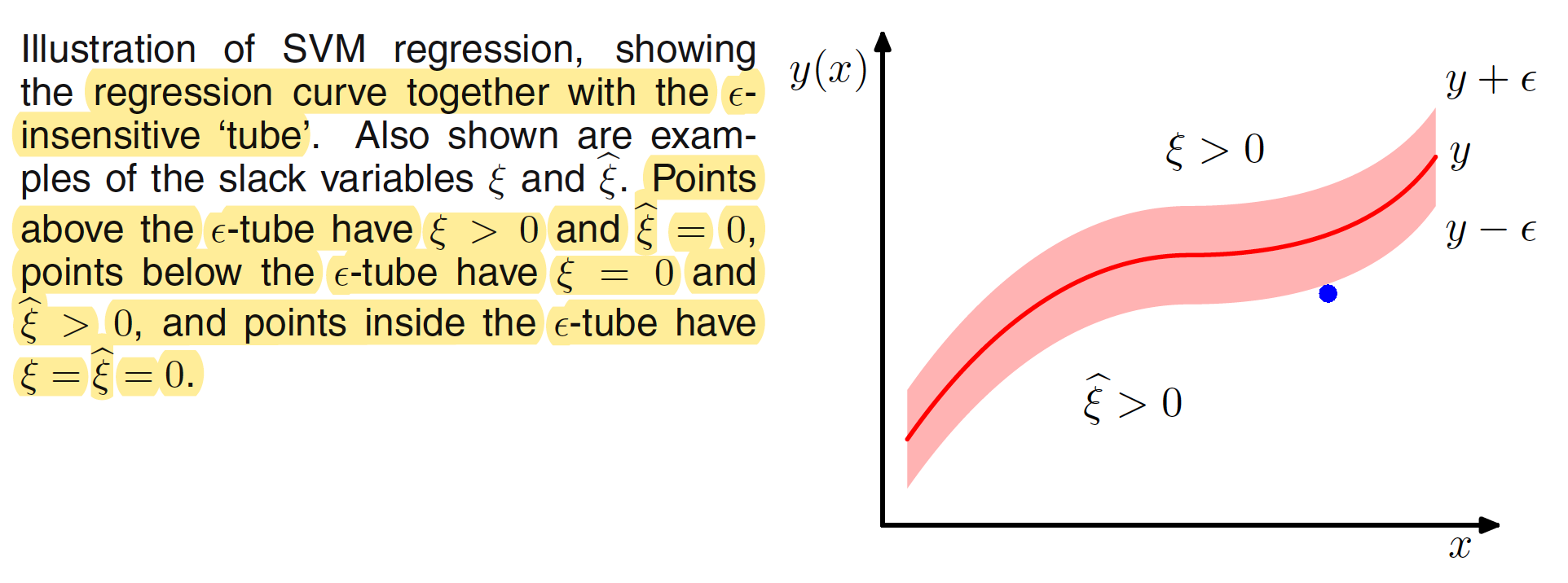
The condition for a target point to lie inside the $\epsilon$-tube is that $y_n - \epsilon \leq t_n \leq y_n + \epsilon$. Introducing the slack variable allows points to lie outside the tube provided the slack variables are nonzero, and the corresponding conditions are
$$\begin{align} t_n \leq y_n + \epsilon + \xi_n \end{align}$$
$$\begin{align} t_n \geq y_n - \epsilon - \xi_n^{’} \end{align}$$
The error function then reduces to
$$\begin{align} C\sum_{n=1}^{N}(\xi_n + \xi_n^{’}) + \frac{1}{2}||W||^2 \end{align}$$
which must be minimized to the constraints $\xi_n \geq 0$, $\xi_n^{’} \geq 0$, $t_n \leq y_n + \epsilon + \xi_n$ and $t_n \geq y_n - \epsilon - \xi_n^{’}$. After introducing Lagrange multiplier $a_n \geq 0$, $a_n^{’} \geq 0$, $\mu_n \geq 0$ and $\mu_n^{’} \geq 0$, the Lagrangian is
$$\begin{align} L = C\sum_{n=1}^{N}(\xi_n + \xi_n^{’}) + \frac{1}{2}||W||^2 - \sum_{n=1}^{N}(\mu_n\xi_n + \mu_n^{’}\xi_n^{’}) - \end{align}$$
$$\begin{align} \sum_{n=1}^{N}a_n(y_n + \epsilon + \xi_n - t_n) - \sum_{n=1}^{N}a_n^{’}(-y_n + \epsilon + \xi_n^{’} + t_n) \end{align}$$
Substituting for $y_n = y(X_n) = W^TX_n + b$ and differentiating with respect to $W,b,\xi_n,\xi_n^{’}$ and equating them to zero, we have
$$\begin{align} \frac{\partial L}{\partial W} = 0 \implies W = \sum_{n=1}^{N} (a_n - a_n^{’})\phi(X_n) \end{align}$$
$$\begin{align} \frac{\partial L}{\partial b} = 0 \implies \sum_{n=1}^{N} (a_n - a_n^{’}) = 0 \end{align}$$
$$\begin{align} \frac{\partial L}{\partial \xi_n} = 0 \implies a_n + \mu_n = C \end{align}$$
$$\begin{align} \frac{\partial L}{\partial \xi_n^{’}} = 0 \implies a_n^{’} + \mu_n^{’} = C \end{align}$$
Using these results to eliminate the corresponding variables from the Lagrangian, we have the dual problem of maximizing
$$\begin{align} L(a,a^{’}) = -\frac{1}{2}\sum_{n=1}^{N}\sum_{m=1}^{N} (a_n - a_n^{’})(a_m - a_m^{’})k(X_n,X_m) \end{align}$$
$$\begin{align} -\epsilon\sum_{n=1}^{N}(a_n + a_n^{’}) + \sum_{n=1}^{N}(a_n - a_n^{’})t_n \end{align}$$
where $k(X,X^{’}) = \phi(X)^T\phi(X^{’})$ The expression for the dual problem is derived the same way as the one in the previous section. The updated constraints for the dual problem are
$$\begin{align} 0 \leq a_n \leq C \end{align}$$
$$\begin{align} 0 \leq a_n^{’} \leq C \end{align}$$
Using the value of $W$, the prediction for the new inputs can be made using
$$\begin{align} y(X) = \sum_{n=1}^{N} (a_n - a_n^{’})k(X,X_n) + b \end{align}$$
The corresponding KKT conditions, which state that at the solution the product of the dual variables and the constraint must vanish, are given by
$$\begin{align} a_n(y_n + \epsilon + \xi_n - t_n) = 0 \end{align}$$
$$\begin{align} a_n^{’}(-y_n + \epsilon + \xi_n^{’} + t_n) = 0 \end{align}$$
$$\begin{align} (C - a_n)\xi_n = 0 \end{align}$$
$$\begin{align} (C - a_n^{’})\xi_n^{’} = 0 \end{align}$$
The support vectors are those data points for which either $a_n \neq 0$ or $a_n^{’} \neq 0$. These are the points that lie on the boundary of the $\epsilon$-tube or outside the tube. All points inside the tube have $a_n=a_n^{’}=0$. We have a sparse solution as the only term that needs to be evaluated are the one that involves the support vectors. Parameter $b$ can be found similarly as
$$\begin{align} b = t_n - \epsilon - W^T\phi(X_n) \end{align}$$
$$\begin{align} b = t_n - \epsilon - \sum_{m=1}^{N} (a_m - a_m^{’})k(X_n,X_m) \end{align}$$
It is better to compute $b$ for each of the support vectors and take the average as discussed in the previous sections.
7.1.5 Computational Learning Theory
Support vector machines have largely been motivated and analysed using a theoretical framework known as computational learning theory, also sometimes called statistical learning theory. A probably approximately correct, or PAC, learning framework is used to understand how large a data set needs to be in order to give good generalization. It also gives bounds for the computational cost of learning. Suppose a dataset $D$ of size $N$ is drawn from some joint distribution $p(X,t)$, and we restrict it to be a noise free situation in which the class labels are determined by some unknown determinitic function $t=g(X)$. In PAC learning we say that a function $f(X;D)$, drawn from a space $F$ of such functions on the basis of the training set $D$, has good generalization if its expected error rate is below some pre-specifie threshold $\epsilon$, so that
$$\begin{align} E_{X,t}[I(f(X;D) \neq t)] < \epsilon \end{align}$$
where $I(.)$ is the indicator function and the expectation is taken with respect to the distribution $p(X,t)$.