5.2 Network Training
A simple approach to the problem of determining the network parameters is to make an analogy with the discussion of polynomial curve fitting, and therefore to minimize a sum-of-squares error function. Given a training set comprising a set of input vectors ${X_n}$, where $n=1,2,…,N$ with the corresponding output set as ${t_n}$, we minimize the error function
$$\begin{align} E(W) = \frac{1}{2}\sum_{n=1}^{N}||y_n(X_n,W) - t_n||^2 \end{align}$$
Let us consider a regression case with single target variable $t$ that can take any real value. We assume that $t$ has a Gaussian distribution with an $X$-dependent mean, which is given by the output of the neural network as
$$\begin{align} p(t|X,W) = N(t|y(X,W),\beta^{-1}) \end{align}$$
where $\beta$ is the precision (inverse variance) of the Gaussia noise. For the case of the data set with $N$ independent and identically distributed observations ${X_n}$, where $n=1,2,…,N$ with the corresponding output set as ${t_n}$, the corresponding likelihood function will be
$$\begin{align} p(t|X,W,\beta) = \prod_{n=1}^{N}N(t_n|y(X_n,W),\beta^{-1}) \end{align}$$
Taking the neagtaive algorithm, the error function is given as
$$\begin{align} \frac{\beta}{2}\sum_{n=1}^{N} \bigg[(y(X_n,W) - t_n)^2\bigg] + \frac{N}{2}\ln(2\pi) - \frac{N}{2}\ln(\beta) \end{align}$$
which can be used to learn the parameters $W$ and $\beta$. Consider first the determination of $W$. Maximizing the likelihood function is equivalent to minimizing the sum-of-squares error function given by
$$\begin{align} E(W) = \frac{1}{2}\sum_{n=1}^{N} (y(X_n,W) - t_n)^2 \end{align}$$
The determined value is denoted by $W_{ML}$ as it is the maximum-likelihood solution. In practice, the nonlinearity of the network function $y(X_n,W)$ causes the error $E(W)$ to be nonconvex, and so in practice local maxima of the likelihood may be found, corresponding to local minima of the error function. Iterative optimizatiion algorithms are used to find the local minima.
Having found $W_{ML}$, the value of $\beta$ can be found by minimizing the negative log likelihood to give
$$\begin{align} \frac{1}{\beta_{ML}} = \frac{1}{N}\sum_{n=1}^{N} (y(X_n,W) - t_n)^2 \end{align}$$
It should be noted that this can be evaluated once the iterative optimization required to find $W_{ML}$ is completed. For the case of $K$ independent target variables, the optimal value of $\beta$ is given as
$$\begin{align} \frac{1}{\beta_{ML}} = \frac{1}{NK}\sum_{n=1}^{N} ||y(X_n,W) - t_n||^2 \end{align}$$
The behaviour of the error function for the regression case is quite simple. For regression problem, the output activation is unit function, i.e. $y_k = a_k$. The differential of error function with respect to output activation is
$$\begin{align} \frac{\partial{E}}{\partial{a_k}} = y_k - t_k \end{align}$$
For a binary classifier having single target variable, the activation function is a logistic sigmoid given as
$$\begin{align} y = \sigma(a) = \frac{1}{1+e^{-a}} \end{align}$$
The output $y(X,W)$ can be interpretted as the probability of class $C_1$, i.e. $p(C_1|X) = y(X,W)$ and $p(C_2|X) = 1 - y(X,W)$. The conditional distribution of target given input follows Bernoulli distribution and is given as
$$\begin{align} p(t|X,W) = y(X,W)^{t}{1 - y(X,W)}^{1-t} \end{align}$$
If we consider a training set of independent observations, then the error function, which is given by the negative log likelihood, is then a cross-entropy error function of the form
$$\begin{align} E(W) = -\sum_{n=1}^{N}{t_n\ln(y_n) + (1-t_n)\ln(1-y_n)} \end{align}$$
where $y_n = y(X_n,W)$. Using the cross-entropy error function instead of the sum-of-squares for a classification problem leads to faster training as well as improved generalization.
If we have $K$ separate binary classifications to perform, then we can use a network having $K$ outputs each of which has a logistic sigmoid activation function. Associated with each output is a binary class label $t_k \in {0,1}$, where $k = 1, . . . , K$. If we assume that the class labels are independent, given the input vector, then the conditional distribution of the targets is
$$\begin{align} p(t|X,W) = \prod_{k=1}^{K}y_k(X,W)^{t_k}{1 - y_k(X,W)}^{1-t_k} \end{align}$$
The corresponding error function is
$$\begin{align} E(W) = -\sum_{n=1}^{N} \sum_{k=1}^{K} {t_{nk}\ln(y_{nk}) + (1-t_{nk})\ln(1-y_{nk})} \end{align}$$
where $y_{nk} = y_k(X_n, W)$.
For standard multiclass classification problem, in which each output is assigned to $K$ mutually exclusive classes, the binary target variables $t_k \in {0,1}$ have a $1-of-K$ encoding scheme indicating the class. The network outputs are interpreted as $y_k(X,W) = p(t_k=1| X)$, leading to following error function
$$\begin{align} E(W) = -\sum_{n=1}^{N} \sum_{k=1}^{K} t_{nk}\ln(y_{nk}) \end{align}$$
The output unit activation function is given by a softmax function as
$$\begin{align} y_k(X,W) = \frac{exp(a_k(X,W))}{\sum_j exp(a_j(X,W))} \end{align}$$
This activation ensures that $\sum_k y_k = 1$.
In summary, there is a natural choice of both output unit activation function and matching error function, according to the type of problem being solved. For regression we use linear outputs and a sum-of-squares error, for (multiple independent) binary classifications we use logistic sigmoid outputs and a cross-entropy error function, and for multiclass classification we use softmax outputs with the corresponding multiclass cross-entropy error function.
5.2.1 Parameter Optimization
The algorithm to find the weight $W$ which minimizes the error function $E(W)$ is discussed in this section. Below figure shows how the error function can be situated in the weight space.
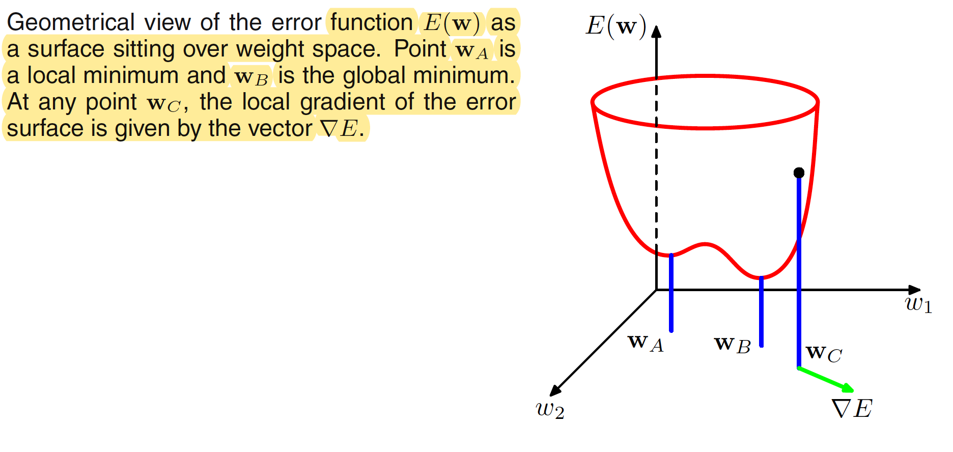
If we make a small step in weight space from $W$ to $W+\delta W$ then the change in the error function is $\delta E \simeq \delta W^T \nabla E(W)$ , where the vector $\nabla E(W)$ points in the direction of greatest rate of increase of the error function. Because the error $E(W)$ is a smooth continuous function of $W$, its smallest value will occur at a point in weight space such that the gradient of the error function vanishes, so that
$$\begin{align} \nabla E(W) = 0 \end{align}$$
as otherwise we could make a small step in the direction of and thereby further reduce the error. Points at which the gradient vanishes are called stationary points, and may be further classified into minima, maxima, and saddle points.
It should be noted that, there will be many points in weight space at which the gradient vanishes (or is numerically very small). For any point w that is a local minimum, there will be other points in weight space that are equivalent minima. For instance, in a two-layer network, with $M$ hidden units, each point in weight space is a member of a family of $M!2M$ equivalent points. A minimum that corresponds to the smallest value of the error function for any weight vector is said to be a global minimum. Any other minima corresponding to higher values of the error function are said to be local minima. For a successful application of neural networks, it may not be necessary to find the global minimum (and in general it will not be known whether the global minimum has been found) but it may be necessary to compare several local minima in order to find a sufficiently good solution.
To find the solution to the equation $\nabla E(W) = 0$, we choose some initial weight $W^{(0)}$ and then move through weight space in a succession of steps of the form
$$\begin{align} W^{(\tau + 1)} = W^{(\tau)} + \Delta W^{(\tau)} \end{align}$$
where $\tau$ labels the iteration step. In order to understand the importance of gradient information, it is useful to consider a local approximation to the error function based on a Taylor expansion.
5.2.2 Local Quadratic Approximation
Consider the Taylor expansion of $E(W)$ around some point $\hat{W}$ in weight space
$$\begin{align} E(W) \simeq E(\hat{W}) + (W - \hat{W})^Tb + \frac{1}{2}(W - \hat{W})^T H (W - \hat{W}) \end{align}$$
where cubic and higher order terms are omitted and
$$\begin{align} b = \nabla E(W)\bigg|_{W = \hat{W}} \end{align}$$
and the Hessian matrix $H=\nabla\nabla E$ has the elements
$$\begin{align} H_{ij} = \frac{\partial E}{\partial w_i \partial w_j}\bigg|_{W = \hat{W}} \end{align}$$
Differentiating the Taylor expansion with respect to $W$, the local approximation of the gradient is given as
$$\begin{align} \nabla \simeq b + H(W - \hat{W}) \end{align}$$
For points $W$ that are sufficiently close to $\hat{W}$, these expressions will give reasonable approximations for the error and its gradient.
5.2.3 Use of Gradient Information
It is possible to evaluate the gradient of an error function efficiently by means of the backpropagation procedure. In the quadratic approximation to the error function using the Taylor expansion, the error surface is specified by the quantities $b$ and $H$, which contain a total of $W(W+1)/2$ independent elements (because the matrix $H$ is symmetric), where $W$ is the dimensionality of $W$ (i.e., the total number of adaptive parameters in the network). The location of the minimum of this quadratic approximation therefore depends on $O(W^2)$ parameters, and we should not expect to be able to locate the minimum until we have gathered $O(W^2)$ independent pieces of information. If we do not make use of gradient information, we would expect to have to perform $O(W^2)$ function evaluations, each of which would require $O(W)$ steps. Thus, the computational effort needed to find the minimum using such an approach would be $O(W^3)$.
With an algorithm that makes use of the gradient information, each evaluation of $\nabla E$ brings $W$ items of information, we might hope to find the minimum of the function in $O(W)$ gradient evaluations. As we shall see, by using error backpropagation, each such evaluation takes only $O(W)$ steps and so the minimum can now be found in $O(W^3)$ steps.
5.2.4 Gradient Descent Optimization
The simplest approach to using gradient information is to choose the weight update to comprise a small step in the direction of the negative gradient, so that
$$\begin{align} W^{(\tau + 1)} = W^{(\tau)} - \eta\nabla E(W^{(\tau)}) \end{align}$$
where $\eta > 0$ is called as the learning rate. Note that the error function is defined with respect to a training set, and so each step requires that the entire training set be processed in order to evaluate $\nabla E$. Techniques that use the whole data set at once are called batch methods. At each step the weight vector is moved in the direction of the greatest rate of decrease of the error function, and so this approach is known as gradient descent or steepest descent.
There is, however, an on-line version of gradient descent that has proved useful in practice for training neural networks on large data sets. Error functions based on maximum likelihood for a set of independent observations comprise a sum of terms, one for each data point and is given as
$$\begin{align} E(W) = \sum_{n=1}^{N}E_n(W) \end{align}$$
On-line gradient descent, also known as sequential gradient descent or stochastic gradient descent, makes an update to the weight vector based on one data point at a time, so that
$$\begin{align} W^{(\tau + 1)} = W^{(\tau)} - \eta\nabla E_n(W^{(\tau)}) \end{align}$$
This update is repeated by cycling through the data either in sequence or by selecting points at random with replacement.
One advantage of on-line methods compared to batch methods is that the former handle redundancy in the data much more efficiently. To see, this consider an extreme example in which we take a data set and double its size by duplicating every data point. Note that this simply multiplies the error function by a factor of 2 and so is equivalent to using the original error function. Batch methods will require double the computational effort to evaluate the batch error function gradient, whereas online methods will be unaffected. Another property of on-line gradient descent is the possibility of escaping from local minima, since a stationary point with respect to the error function for the whole data set will generally not be a stationary point for each data point individually.