One of the major limitations of the modeling techniques discussed so far is the way fixed basis functions are used to defind the transformation of data points. This approach leads to a much sparser models. An alternative approach is to fix the number of basis functions in advance but allow them to be adaptive, in other words to use parametric forms for the basis functions in which the parameter values are adapted during training. The most successful model of this type in the context of pattern recognition is the feed-forward neural network, also known as the multilayer perceptron. The resulting model is significantly more compact and hence faster to evaluate. The price to be paid for this compactness is that the likelihood function, which forms the basis for network training, is no longer a convex function of the model parameters.
5.1 Feed-forward Network Functions
The linear models for regression and classification are based on linear combinations of fixed nonlinear basis functions $\phi_j(X)$ and take the form
$$\begin{align} y(X,W) = f\bigg(\sum_{j=1}^{M} W_j\phi_j(X)\bigg) \end{align}$$
where $f(.)$ is a nonlinear activation function in the case of classification and is the identity in the case of regression. Our goal is to extend this model by making the basis function $\phi_j(X)$ depend on parameters and then allow these parameters to be adjusted along with the weights $W$ during the training process. In neural networks, each basis function is a nonlinear functiin of a linear combination of the inputs, where the coefficients in the linear combination are adaptive parameters.
In a neural network with one hidden layer, we first construct $M$ linear combinations of the input variables $X_1,X_2,…,X_D$ as
$$\begin{align} a_j = \sum_{i=0}^{D}w_{ji}^{(1)}X_i \end{align}$$
where we have included the bias term with input as $1$. $j=1,2,…,M$ denotes the total number of neurons or connections in the next layer. The superscript $(1)$ denotes the first layer (input layer) of the network. The quantities $a_j$ are known as the activations which are transformed using a differentiable nonlinear activation function $h(.)$ as
$$\begin{align} z_j = h(a_j) \end{align}$$
These values are again combined post the hidden layer to give the output unit activations as
$$\begin{align} a_k = \sum_{j=0}^{M}w_{kj}^{(2)}z_j \end{align}$$
$k=1,2,…,K$ denotes the total number of units or neurons in the output layer. Finally the output unit activations are transformed using the appropriate activation function to give the outputs $y_k$. For standard regression problem, unit activation is used, i.e $y_k = a_k$. For binary classification problems, each output unit activation is transformed using a logistic sigmoid function so that
$$\begin{align} y_k = \sigma(a_k) \end{align}$$
where
$$\begin{align} \sigma(a) = \frac{1}{1+exp(-a)} \end{align}$$
For multiclass problems, a softmax activation function is used. It should be noted that $a_i$ is the activartion unit for layer $i$. The weight connecting layer $j$ and $i$ is denoted as $w_{ji}$.. These stages can be combined together to give
$$\begin{align} y_k(X,W) = \sigma\bigg(\sum_{j=0}^{M}w_{kj}^{(2)}h\bigg(\sum_{i=0}^{D}w_{ji}^{(1)}X_i\bigg)\bigg) \end{align}$$
Thus the neural network model is simply a nonlinear function from a set of input variables ${X_i}$ to a set of output variables ${y_k}$ controlled by a vector $W$ of adjustable parameters. The pictorial representation of the above neural network model is shown below
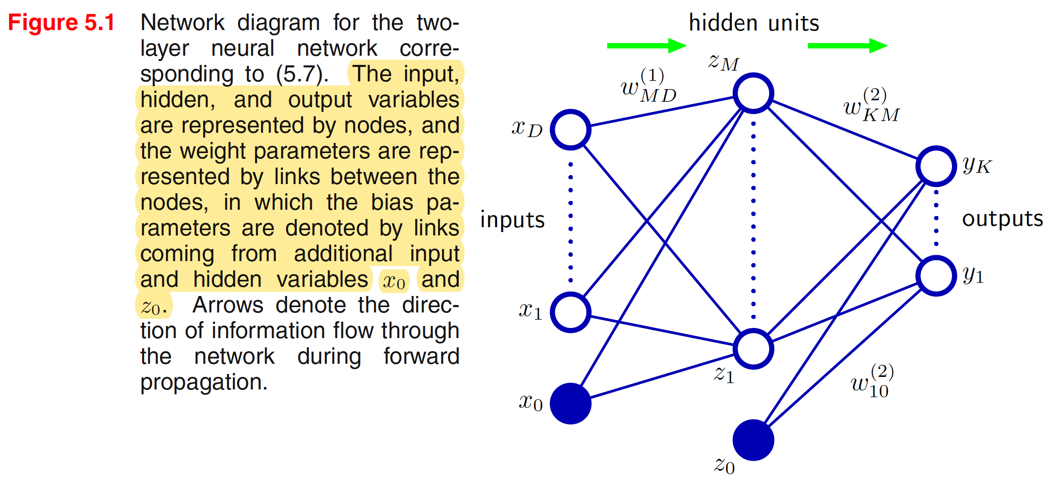
The neural network model comprises two stages of processing, each of which resembles the perceptron model. A key difference compared to the perceptron, however, is that the neural network uses continuous sigmoidal nonlinearities in the hidden units, whereas the perceptron uses step-function nonlinearities. This means that the neural network function is differentiable with respect to the network parameters, and this property will play a central role in network training. If the activation functions of all the hidden units in a network are taken to be linear, then for any such network we can always find an equivalent network without hidden units. This follows from the fact that the composition of successive linear transformations is itself a linear transformation. For the network show in above figure, we recommend a terminology in which it is called a two-layer network, because it is the number of layers of adaptive weights that is important for determining the network properties.
Because there is a direct correspondence between a network diagram and its mathematical function, we can develop more general network mappings by considering more complex network diagrams. However, these must be restricted to a feed-forward architecture, in other words to one having no closed directed cycles, to ensure that the outputs are deterministic functions of the inputs.
5.1.1 Weight-space Symmetries
One property of feed-forward networks, which will play a role when we consider Bayesian model comparison, is that multiple distinct choices for the weight vector $W$ can all give rise to the same mapping function from inputs to outputs. For example, if we change the sign of all of the weights and the bias feeding into a particular hidden unit, then, for a given input pattern, the sign of the activation of the hidden unit will be reversed (if we have an odd activation function). This transformation can be exactly compensated by changing the sign of all of the weights leading out of the same hidden unit. So, we have found two different weight vectors that give rise to the same mapping function. For $M$ hidden units, we will have a total of $M$ such sign-flips, and hence any given weight vector will be one of the set $2^M$ equivalent weight vectors.
Similarly, imagine that we interchange the values of all of the weights (and the bias) leading both into and out of a particular hidden unit with the corresponding values of the weights (and bias) associated with a different hidden unit. Again, this clearly leaves the network input–output mapping function unchanged, but it corresponds to a different choice of weight vector. For $M$ hidden units, we can have a total of $M!$ such combinations. Hence, a network with $M$ hidden units will have an overall weight-space symmetry factor of $M!2^M$.