5.3 Error Backpropagation
Our goal in this section is to find an efficient technique for evaluating the gradient of an error function $E(W)$ for a feed-forward neural network. We shall see that this can be achieved using a local message passing scheme in which information is sent alternately forwards and backwards through the network and is known as error backpropagation, or sometimes simply as backprop.
Most training algorithms involve an iterative procedure for minimization of an error function, with adjustments to the weights being made in a sequence of steps. At each such step, we can distinguish between two distinct stages.
-
In the first stage, the derivatives of the error function with respect to the weights must be evaluated. As we shall see, the important contribution of the backpropagation technique is in providing a computationally efficient method for evaluating such derivatives. Because it is at this stage that errors are propagated backwards through the network, we shall use the term backpropagation specifically to describe the evaluation of derivatives.
-
In the second stage, the derivatives are then used to compute the adjustments to be made to the weights.
5.3.1 Evaluation of Effor-function Derivatives
We now derive the backpropagation algorithm for a general network having arbitrary feed-forward topology, arbitrary differentiable nonlinear activation functions, and a broad class of error function.
Many error functions of practical interest, for instance those defined by maximum likelihood for a set of i.i.d. data, comprise a sum of terms, one for each data point in the training set, so that
$$\begin{align} E(W) = \sum_{n=1}^{N}E_n(W) \end{align}$$
Here we shall consider the problem of evaluating $\nabla E_n(W)$. This may be used directly for sequential optimization, or the results can be accumulated over the training set in the case of batch methods.
In a simple linear model, the outputs $y_k$ are linear combination of the input variables $X_i$ so that
$$\begin{align} y_k = \sum_{i} W_{ki}X_i \end{align}$$
The error function for a particular input pattern takes the form
$$\begin{align} E_n = \frac{1}{2}\sum_{k} (y_{nk} - t_{nk})^2 \end{align}$$
where $y_{nk} = y_k(X_n,W)$. The gradient of this error function with respect to a weight $W_{ji}$ is given as
$$\begin{align} \frac{\partial E_n}{\partial W_{ji}} = (y_{nj} - t_{nj})X_{ni} \end{align}$$
This derivative is interpreted as: $W_{ji}$ connects the output neuron $j$ and input neuron $i$. The derivative is a mutiple of error at the output neuron $y_{nj} - t_{nj}$ and the input signal $X_{ni}$ at the input neuron. A typical feedforward network with two connected neurons is shown below.
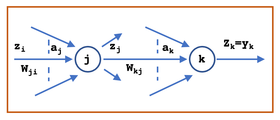
The input to unit $j$ is the weighed sum of the activations of unit $i$ (output from the neurons in the previous layer) and is given as
$$\begin{align} a_j = \sum_{i} W_{ji}z_i \end{align}$$
where $W_{ji}$ is the weight associated with the connection from unit $i$ to unit $j$. The activation $z_j$ of unit $j$ is then computed using non-inear transformation function $h(.)$, also called as activation function as
$$\begin{align} z_j = h(a_j) \end{align}$$
For each pattern in the training set, we shall suppose that we have supplied the corresponding input vector to the network and calculated the activations of all of the hidden and output units in the network by successive application of the above equations. This process is often called forward propagation because it can be regarded as a forward flow of information through the network.
Now consider the evaluation of the derivative of $E_n$ with respect to a weight $W_{ji}$. $E_n$ depends on the weight $W_{ji}$ only through the summed up input $a_j$ to unit $j$. From chain rule, we have
$$\begin{align} \frac{\partial E_n}{\partial W_{ji}} = \frac{\partial E_n}{\partial a_{j}}\frac{\partial a_j}{\partial W_{ji}} = \delta_j z_i \end{align}$$
where $\delta_j = \frac{\partial E_n}{\partial a_{j}}$ are referred to as the error at unit $j$ and $z_i$ is the activation of unit $i$. The derivative is obtained simply by multiplying the value of error $\delta$ for the unit at the output end of the weight by the value of activation $z$ for the unit at the input end of the weight. Hence, we need only to calculate the value of the errors $\delta_j$ for each hidden and output unit in the network.
For the output unit $k$ with unit activation function, we have $y_k = a_k$ and with a sum-of-square error, the error at unit $k$ is
$$\begin{align} E_n = \frac{1}{2} (y_{nk} - t_{nk})^2 \end{align}$$
This gives us the value of $\delta_k$ (last expression is obtained simply by omitting the subscript $n$) as
$$\begin{align} \delta_k = \frac{\partial E_n}{\partial a_{k}} = y_{nk} - t_{nk} = y_{k} - t_{k} \end{align}$$
For any hidden unit (consider the unit $j$), the error will back-propagate from all the neurons/units in the next layer to which it sends the connection. Using chain rule of partial derivative, we have
$$\begin{align} \delta_j = \frac{\partial E_n}{\partial a_{j}} = \sum_{k} \frac{\partial E_n}{\partial a_{k}} \frac{\partial a_k}{\partial a_{j}} = \sum_{k} \delta_k \frac{\partial a_k}{\partial a_{j}} \end{align}$$
We further have
$$\begin{align} a_k = W_{kj}z_j = W_{kj}h(a_j) \end{align}$$
and hence
$$\begin{align} \frac{\partial a_k}{\partial a_{j}} = W_{kj}h^{’}(a_j) \end{align}$$
This gives us
$$\begin{align} \delta_j = \sum_{k} \delta_k \frac{\partial a_k}{\partial a_{j}} = h^{’}(a_j)\sum_{k} \delta_k W_{kj} \end{align}$$
This tells us that the value of $\delta$ for a particular hidden unit can be obtained by propagating the $\delta$’s backwards from units higher up in the network.
5.3.2 A Simple Example
Consider a two-layer network of the form illustrated above, together with a sum-of-squares error, in which the output units have linear activation functions, so that $y_k = a_k$, while the hidden units have logistic sigmoid activation functions given by
$$\begin{align} h(a) = \tanh{(a)} = \frac{e^a - e^{-a}}{e^a + e^{-a}} \end{align}$$
For the activation function, we have
$$\begin{align} h^{’}(a) = 1 - h(a)^2 \end{align}$$
The error $\delta$’s for the output unit is given as
$$\begin{align} \delta_k = y_{k} - t_{k} \end{align}$$
where $y_k$ is the activation of output unit $k$, and $t_k$ is the corresponding target, for a particular input pattern $X_n$.
For the hidden units, the backpropagated error is given as
$$\begin{align} \delta_j = h^{’}(a_j)\sum_{k} \delta_k W_{kj} = (1 - h(a_j)^2) \sum_{k} \delta_k W_{kj} = (1 - z_j)^2 \sum_{k} \delta_k W_{kj} \end{align}$$
Finally, the derivatives with respect to the hidden and output layer is given as
$$\begin{align} \frac{\partial E_n}{\partial W_{ji}^{(h)}} = \delta_j X_i \end{align}$$
$$\begin{align} \frac{\partial E_n}{\partial W_{kj}^{(o)}} = \delta_k z_j \end{align}$$
5.3.3 The Jacobian Matrix
The technique of backpropagation can also be applied to the calculation of other derivatives. Here we consider the evaluation of the Jacobian matrix, whose elements are given by the derivatives of the network outputs with respect to the inputs
$$\begin{align} J_{ki} = \frac{\partial y_k}{\partial X_i} \end{align}$$
where each such derivative is evaluated with all other inputs held fixed. Because the Jacobian matrix provides a measure of the local sensitivity of the outputs to changes in each of the input variables, it also allows any known errors $\Delta X_i$ associated with the inputs to be propagated through the trained network in order to estimate their contribution $\Delta y_k$ to the errors at the outputs, through the relation
$$\begin{align} \Delta y_k \simeq \sum_{i} \frac{\partial y_k}{\partial X_i} \Delta X_i \end{align}$$
which is valid provided the $|\Delta X_i|$ are small. The Jacobian can be computed as
$$\begin{align} J_{ki} = \frac{\partial y_k}{\partial X_i} = \sum_{j} \frac{\partial y_k}{\partial a_j} \frac{\partial a_j}{\partial X_i} = \sum_{j} W_{ji} \frac{\partial y_k}{\partial a_j} \end{align}$$
It should be noted that the sum is taken over all the units $j$ which are fed by the input $X_i$. Next we have to compute $\frac{\partial y_k}{\partial a_j}$. It can be computed as
$$\begin{align} \frac{\partial y_k}{\partial a_j} = \sum_{l} \frac{\partial y_k}{\partial a_l} \frac{\partial a_l}{\partial a_j} = \sum_{l} \frac{\partial y_k}{\partial a_l} W_{lj} h^{’}(a_j) = h^{’}(a_j) \sum_{l} W_{lj} \frac{\partial y_k}{\partial a_l} \end{align}$$
where the sum is taken over all units $l$ to which the unit $j$ sends connection. $\frac{\partial y_k}{\partial a_l}$ can be computed using output activation function.