4.1 Discriminant Functions
A discriminant is a function which takes the input vector $X$ and assigns it to one of the classes $C_k$. When the decision surfaces are hyperplanes, we call them as linear discriminants.
4.1.1 Two Classes
The simplest representation of linear discriminant function is
$$\begin{align} y(X) = W^TX + W_0 \end{align}$$
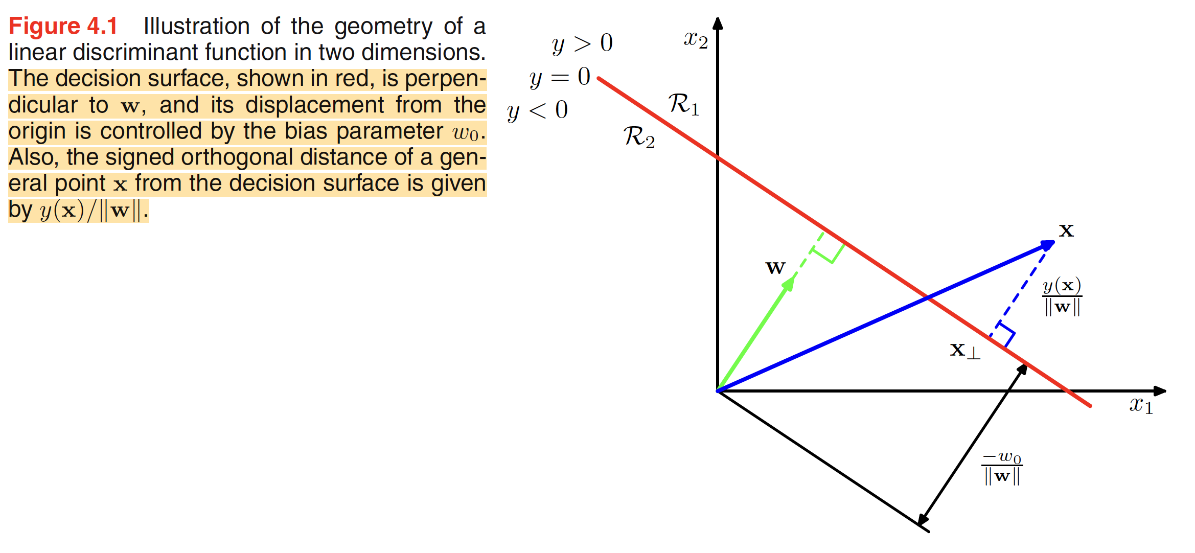
where $W$ is called the weight vector and $W_0$ is bias. The negative of the bias is called threshold. The input vector will be assigned to the class $C_1$ if $y(X) \geq 0$ and $C_2$ otherwise. The decision boundary will be defined by the relation $y(X) = 0$. Let $X_A,X_B$ are the two points lying on the decision surface, then $y(X_A) = y(X_B) = 0$ and hence $W^T(X_A - X_B) = 0$. This means that the weight vector $W$ is orthogonal to every vector in the decision surface, i.e. $W$ determines the direction of the decision surface. Let $X$ be a point on the decsion surface which is closest to the origin. Thie means that this point can be represented as $X = \alpha W$ as the perpendicular weight vector $W$ will be the direction in which we will have the smallest vector passing through origin and the hyperplace. As $X$ lies on the hyperplace, we have $y(X) = W^TX + W_0 = 0$, i.e. $W^TX + W_0 = \alpha W^TW + W_0 = 0$ and hence $\alpha = -W_0/||W||^2$. The distance of the point $X$ from the origin is $||X|| = ||\alpha W|| = \frac{-W_0}{||W||^2}||W|| = \frac{-W_0}{||W||}$. Hence, the normal distance of the hyperplane from the origin is given by $\frac{-W_0}{||W||}$. This means that the bias parameter $W_0$ decides the location of the decision surface.
Another thing to note is that the value of $y(X)$ gives the signed measure of the perpendicular distance $r$ of point $X$ from the decision surface. Let $X_{\perp}$ be the orthogonal projection of $X$ on the decision surface, then
$$\begin{align} X = X_{\perp} + r\frac{W}{||W||} \end{align}$$
as $\frac{W}{||W||}$ is the unit vector which is perpendicular to the decision surface. Multiplying both sides by $W^T$ and adding $W_0$, we have
$$\begin{align} W^TX + W_0 = W^TX_{\perp} + rW^T\frac{W}{||W||} + W_0 \end{align}$$
$$\begin{align} y(X) = y(X_{\perp}) + rW^T\frac{W}{||W||} = rW^T\frac{W}{||W||} = r\frac{||W||^2}{||W||} = r||W|| \end{align}$$
$$\begin{align} r = \frac{y(X)}{||W||} \end{align}$$
The geometrical representation of the result is shown in the below figure.
We can combine the bias into weight vector with the new weight vector represented as $\tilde{W} = (W_0, W)$ with the updated input vector as $\tilde{X} = (1,X)$ and the updated equation
$$\begin{align} y(X) = \tilde{W}^T\tilde{X} \end{align}$$
4.1.2 Multiple Classes
A $K$-class discriminant ($K>2$) can be built by combining multiple two-class discriminant functions. However, there are some limitations to it. Consider a one-versus-the-rest classifier which seperates a particulae class $C_k$ from points not in the class. For a $K$-class problem, we will need a total of $K-1$ classifiers of such kind. The result of this kind of classifiere is shown in the below figure. As shown in the left image, the green region is classified both as class $C_1$ and $C_2$ and hence this region is ambiguously classified.
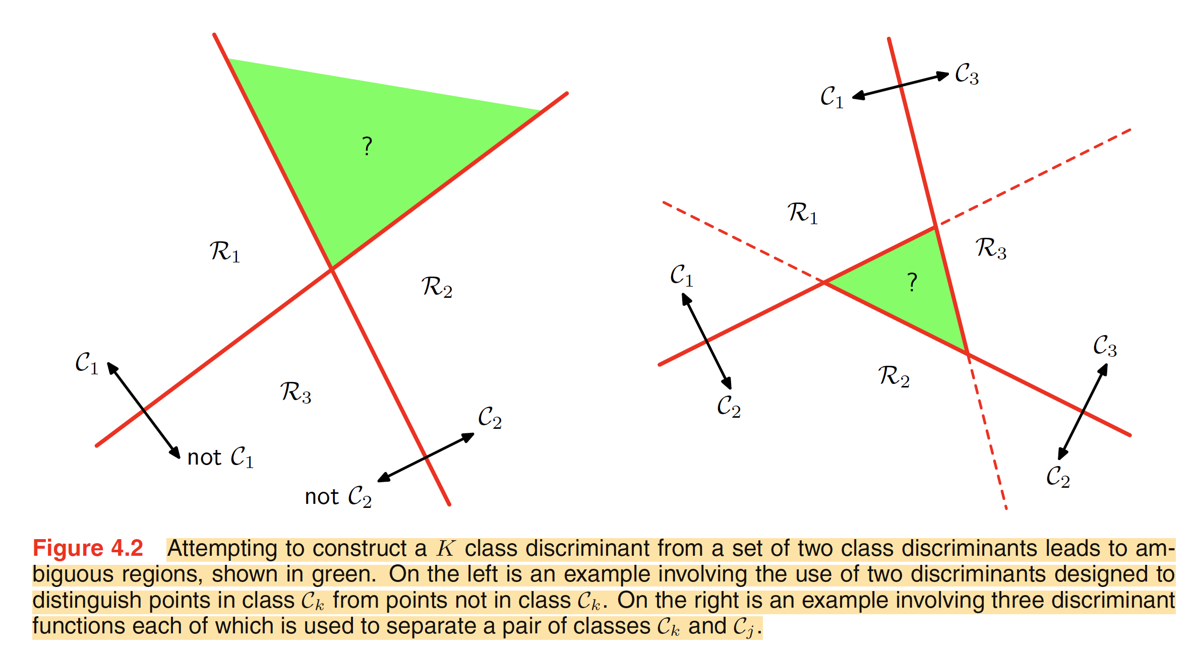
Another approach is to use $K(K-1)/2$ discriminant functions, one for each class pair of classes. This is called as one-versus-one classifier. Each point then can be classified according to the majority vote amongst the discriminant functions. The right hand side image in the above figure shows this approach. The green region has one vote for each of the classes $C_1,C_2$ and $C_3$ and hence being ambiguous.
These ambiguous classification regions can be avoided by using a single $K$-class discriminant comprising of $K$ linear functions of the form
$$\begin{align} y_k(X) = W_{k}^TX + W_{k0} \end{align}$$
The class assignment will be done on the basis of: assign a point $X$ to class $C_k$ if $y_k(X) > y_j(X)$ for all $j \neq k$. The decision boundary between class $C_k$ and $C_j$ is given by $y_k(X) = y_j(X)$ and corresponds to a $(D-1)$-dimensional hyperplane defined by
$$\begin{align} (W_{k} - W_{j})^TX + (W_{k0} - W_{j0}) = 0 \end{align}$$
The decision boundry is same as the one for a two-class case. The decision region of such a discriminant function are always singly connected and convex. For two points $X_A,X_B$ which lie in the decision region $R_k$, any point $\bar{X}$ which lies on the line connecting $X_A,X_B$ can be expressed in the form
$$\begin{align} \bar{X} = \lambda X_A + (1-\lambda)X_B \end{align}$$
From the linearlity of discriminant function
$$\begin{align} y_k(\bar{X}) = \lambda y_k(X_A) + (1-\lambda) y_k(X_B) \end{align}$$
As both $X_A,X_B$ lie inside $R_k$, it follows $y_k(X_A) > y_j(X_A)$ and $y_k(X_B) > y_j(X_B)$ for all $j \neq k$. From this, we get $y_k(\bar{X}) > y_j(\bar{X})$, and hence $\bar{X}$ lies in the region $R_k$. This means that the region $R_k$ is singly connected and convex.