4.1.3 Least Squares for Classification
For the regression problem, minimizing the sum of squares error function led to a simple closed form solution for the parameters. We can check whether the same can be applied to the classification problem in hand. Consider a general classification problem with $K$ classes with a $1-of-K$ binary coding scheme for the target variable $t$. Each class $C_k$ is described by its own linear model given as
$$\begin{align} y_k(X) = W_{k}^TX + W_{k0} \end{align}$$
where $k=1,2,3,…,K$. These can be grouped together in the vector form as
$$\begin{align} y(X) = \tilde {W^T} \tilde{X} \end{align}$$
where the $k^{th}$ column of $\tilde{W}$ corresponds the $k^{th}$ weigth vector $\tilde{W_k}$ and $\tilde{X}$ is a colum vector having the augumented input. The transpose of $\tilde{W}$ will have weight vectors as its rows and hence each entry in the output $y(X) = \tilde {W^T} \tilde{X}$ will have the weight vector multiplied by the input vector for each of the classes ($y_k(X) = \tilde {W_k^T} \tilde{X}$). The input $X$ will be assigned to the class for which $y_k(X) = \tilde {W_k^T} \tilde{X}$ is largest.
Consider a training data having $N$ input output pairs ${X_n,t_n}$ where each $X_n$ will be a $D$-dimensional column vector. The augumented input vector $\tilde{X_n}$ will be a $(D+1)$-dimensional column vector with $1$ appended for the bias. The output vector $t_n$ will be a $K$-dimensional column vector where each entry represents a $0,1$ value based on the class to which the input $X_n$ belongs. Let $T$ be the matrix representing the combined output vector where each row is the transposed output vector $t_n^T$. Let the augumented input vectors when combined together as a matrix form is represented as $\chi$ where rows of $\chi$ are the transposed augumented input $\tilde{X_n}^T$, i.e.
$$\begin{align} \chi = \begin{bmatrix} \tilde{X_1}^T \\ \tilde{X_2}^T \\ … \\ \tilde{X_N}^T \end{bmatrix}_{N \times (D+1)} \end{align}$$
As described earlier, the augumented weight vector $\tilde{W}$ (including bias) will have individual class weights as its column and is represented as
$$\begin{align} \tilde{W} = \begin{bmatrix} W_1 & W_2 & … W_K \end{bmatrix}_{(D+1) \times K} \end{align}$$
The matrix $\chi\tilde{W}$ can be given as
$$\begin{align} \chi\tilde{W} = \begin{bmatrix} \tilde{X_1}^TW_1 & \tilde{X_1}^TW_2 & … & \tilde{X_1}^TW_K \\ \tilde{X_2}^TW_1 & \tilde{X_2}^TW_2 & … & \tilde{X_2}^TW_K \\ … & … & … & …\\ \tilde{X_N}^TW_1 & \tilde{X_N}^TW_2 & … & \tilde{X_N}^TW_K \end{bmatrix}_{N \times K} \end{align}$$
If we offset subtract the output vector from the above matrix, we have
$$\begin{align} \chi\tilde{W} - T = \begin{bmatrix} \tilde{X_1}^TW_1 - t_{11} & \tilde{X_1}^TW_2 - t_{12} & … & \tilde{X_1}^TW_K - t_{1K}\\ \tilde{X_2}^TW_1 - t_{21} & \tilde{X_2}^TW_2 - t_{22} & … & \tilde{X_2}^TW_K - t_{2K}\\ … & … & … & …\\ \tilde{X_N}^TW_1 - t_{N1} & \tilde{X_N}^TW_2 - t_{N2} & … & \tilde{X_N}^TW_K - t_{NK} \end{bmatrix}_{N \times K} \end{align}$$
Considering $(\chi\tilde{W} - T)^T(\chi\tilde{W} - T)$ and just focusing on its diagonal elements, we have
$$\begin{align} (\chi\tilde{W} - T)^T(\chi\tilde{W} - T) = \begin{bmatrix} \sum_{n=1}^{N}(\tilde{X_n}^TW_1 - t_{n1})^2 & & & \\ & \sum_{n=1}^{N}(\tilde{X_n}^TW_2 - t_{n2})^2 & & \\ & & … & \\ & & & \sum_{n=1}^{N}(\tilde{X_n}^TW_K - t_{nK})^2 \end{bmatrix}_{K \times K} \end{align}$$
If we take the trace of the above matrix and divide it by $2$, we have
$$\begin{align} \frac{1}{2}Tr\bigg((\chi\tilde{W} - T)^T(\chi\tilde{W} - T)\bigg) = \frac{1}{2}\sum_{k=1}^{K}\sum_{n=1}^{N}(\tilde{X_n}^TW_k - t_{nk})^2 \end{align}$$
$$\begin{align} = \frac{1}{2}\sum_{n=1}^{N}\sum_{k=1}^{K}(\tilde{X_n}^TW_k - t_{nk})^2 \end{align}$$
The quantity $(\tilde{X_n}^TW_k - t_{nk})^2$ can be viewed as how much the output for $X_n$ for class $C_k$ deviates from the desired output $t_k$. The sum $\sum_{k=1}^{K}(\tilde{X_n}^TW_k - t_{nk})^2$ is the total deviation (combined for all the classes) for the input $X_n$. When this is summed over all teh data points, we get the desired sum-of-squares error. Hence, $\frac{1}{2}Tr\bigg((\chi\tilde{W} - T)^T(\chi\tilde{W} - T)\bigg)$ needs to be minimzed with respect to $\tilde{W}$ to get the optimal parameter. Taking derivative with respect to $\tilde{W}$ and equating it to $0$, we get the optimized solution as
$$\begin{align} \tilde{W} = (\tilde{\chi}^T\chi)^{-1}\chi^TT = \chi^{\dagger}T \end{align}$$
where $\chi^{\dagger}$ is the pseudo-inverse of $\chi$.
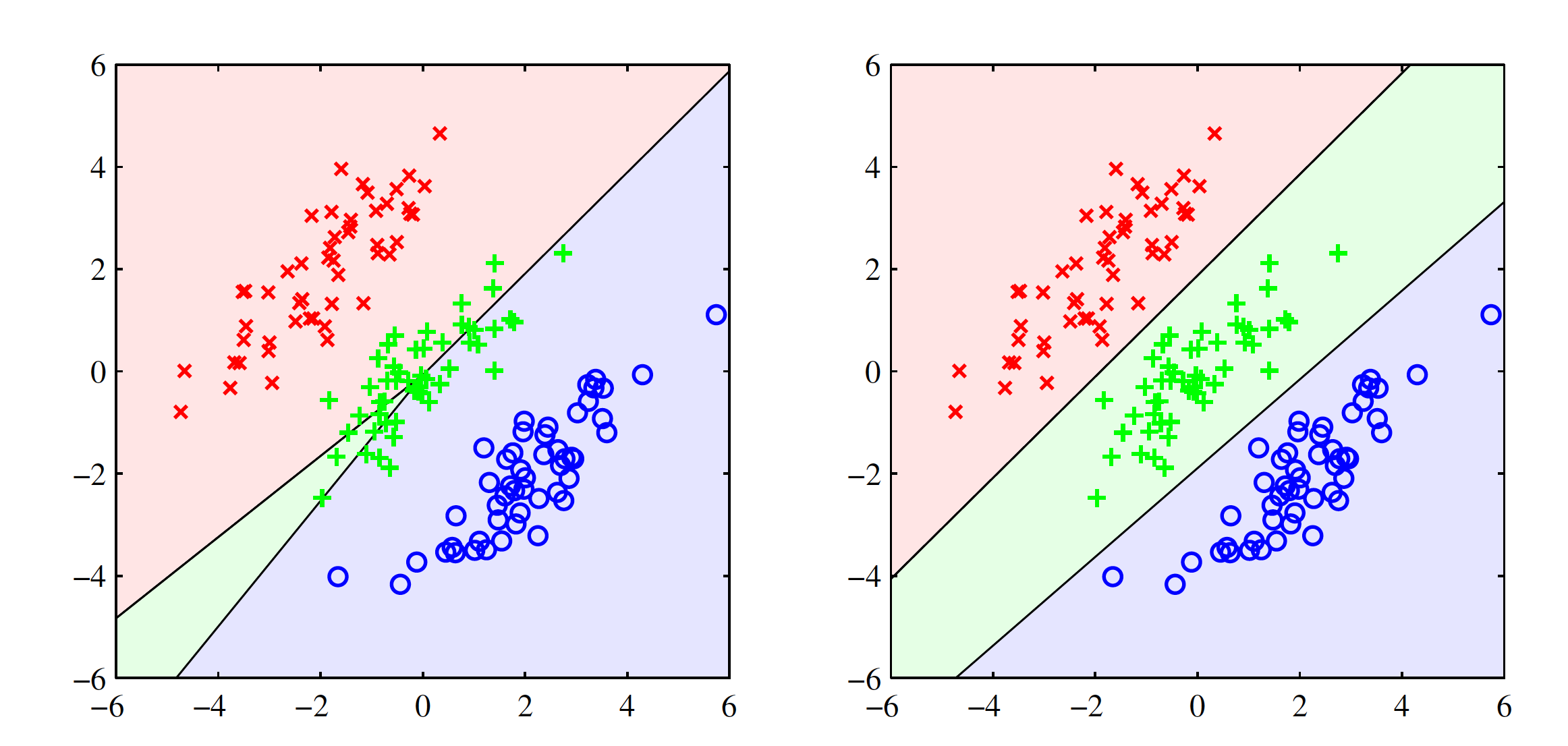
The least square solutions lack the robustness to the outliers and this stands for the classification problem as well. Introducing outliers in the data set changes the decision boundary significantly as the sum-of-squares error penalizes the prediction based on how far they lie from the decision boundary. Least square solution gives poor result even on clear linearly separable data sets. One example in shown in the below figure. Left hand size image shows the output for least squares solution where a lot of gree points are misclassified. Right hand side image shows the output for logistic regression and it works well. The failure of least squares should not surprise us when we recall that it corresponds to maximum likelihood under the assumption of a Gaussian conditional distribution, whereas binary target vectors clearly have a distribution that is far from Gaussian.