2.2 Multinomial Variables
A multinomila variable can be in any of $K$ states instead of just $2$ (in case of a binary variable). For example, a multinomial variable having $K=5$ states can be represented as $x=(0,0,1,0,0)^T$ where it is in a state where $x_3=1$. This vector will satisfy $\sum_{k=1}^K = 1$. If we denote the probability of $x_k=1$ by $\mu_k$, the distribution of $x$ is given as:
$$\begin{align} p(x|\mu) = \prod_{k=1}^{K} \mu_k^{x_k} \end{align}$$
where $\mu = (\mu_1, \mu_2, …, \mu_k)^T$ and $\mu_k \geq 0$ and $\sum_{k}\mu_k = 1$. This distribution can be considered as the generalization of bernoulli distribution for more than $2$ outcomes. This distribution is normalized as (only one of the $x_k=1$ for all $x$):
$$\begin{align} \sum_{x}p(x|\mu) = \sum_{x} \bigg( \prod_{k=1}^{K} \mu_k^{x_k} \bigg) = \sum_{k=1}^{K} \mu_k = 1 \end{align}$$
Expected value of $x$ is given by
$$\begin{align} E[x|\mu] = \sum_{x}p(x|\mu)x = \sum_{x} \bigg( \prod_{k=1}^{K} \mu_k^{x_k} \bigg)x = (\mu_1, \mu_2, …, \mu_M)^T = \mu \end{align}$$
Consider a dataset $D$ of $N$ independent observations $x_1, x_2, …, x_N$. The corresponding likelihood function is given as:
$$\begin{align} p(D|\mu) = \prod_{n=1}^{N}\prod_{k=1}^{K} \mu_{k}^{x_{nk}} \end{align}$$
where $x_{nk}$ is the $k^{th}$ state of $n^{th}$ data point. The expression reduces further to
$$\begin{align} p(D|\mu) = \prod_{n=1}^{N}\prod_{k=1}^{K} \mu_{k}^{x_{nk}} = \prod_{k=1}^{K} \mu_{k}^{(\sum_{n}x_{nk})} = \prod_{k=1}^{K} \mu_{k}^{m_k} \end{align}$$
where $m_k$ represents the number of observations for which $x_k=1$ and is
$$\begin{align} m_k = \sum_{n}x_{nk} \end{align}$$
These are called the sufficient statistics for this distribution. In order to find the maximum likelihood estimate for $\mu$, we need to maximize $\ln p(D|\mu)$ with respect to $\mu_k$ with a constraint $\sum_{k}\mu_k = 1$. This can be achieved using a Lagrange multiplier $\lambda$ and maximizing
$$\begin{align} \sum_{k=1}^{K}m_k \ln \mu_{k} + \lambda \bigg( \sum_{k}^{K}\mu_k - 1\bigg) \end{align}$$
Taking derivative with respect to $\mu_{k}$ and equating it to $0$, we get
$$\begin{align} \frac{m_k}{\mu_{k}} + \lambda = 0 \implies \mu_{k} = \frac{-m_k}{\lambda} \end{align}$$
Substituting the value of $\mu_k$ into the constraint $\sum_{k}\mu_k = 1$, we get
$$\begin{align} \sum_{k}^{K}\frac{-m_k}{\lambda} = 1 \implies \frac{-1}{\lambda}\sum_{k}^{K}m_k = 1 \end{align}$$
$$\begin{align} \implies \frac{-1}{\lambda}N = 1 \implies \lambda = -N \end{align}$$
Hence, we get
$$\begin{align} \mu_{k}^{ML} = \frac{m_k}{N} \end{align}$$
which is the fraction of the $N$ observations for which $x_k=1$. The multinomial distribution which is the distribution of the quantities $m_1,m_2, …, m_K$ conditioned on the parameters $\mu,N$ is given as:
$$\begin{align} Mult(m_1,m_2,…,m_K|\mu,N) = {N \choose m_1m_2…m_K} \prod_{k=1}^{K} \mu_k^{m_k} \end{align}$$
The normalization coefficient is number of ways of partitioning $N$ objects into $K$ groups of size $m_1,m_2,…,m_K$ and is given as
$$\begin{align} {N \choose m_1m_2…m_K} = \frac{N!}{m_1!m_2!…m_K!} \end{align}$$
2.2.1 Dirichlet Distribution
The conjugate prior for the multinomial distribution takes the form
$$\begin{align} p(\mu|\alpha) \propto \prod_{k=1}^{K} \mu_{k}^{\alpha_k - 1} \end{align}$$
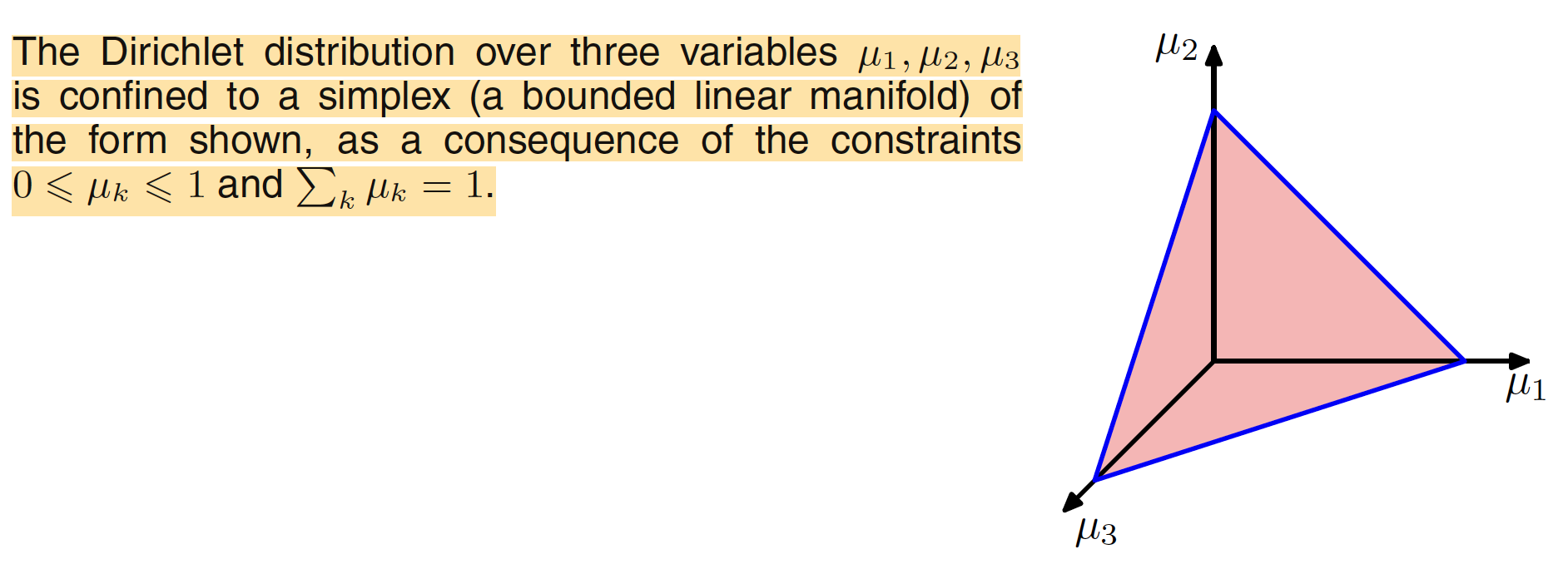
where $0 \leq \mu_k \leq 1$; $\sum_{k} \mu_k = 1$ and $\alpha_1,\alpha_2,…,\alpha_k$ are the parameters of the distribution with $\alpha = (\alpha_1,\alpha_2,…,\alpha_k)^T$. This distribution is called as Dirichlet distribution. It is a mutivariate generalization of beta distribution and hence is also called as multivariate beta distribution. Due to the summation constraint, the ditribution over the space of the ${\mu_k}$ is confined to a simplex of dimensionality $K-1$. For $K=3$, the illustration is shown in the following figure. For the case $K=3$, we have ${\mu_1, \mu_2,\mu_3}$ with constraint $\mu_k \geq 0$ and $\mu_1+\mu_2+\mu_3=1$. These constraints confine the values of $\mu_k$ is the plane shown below.
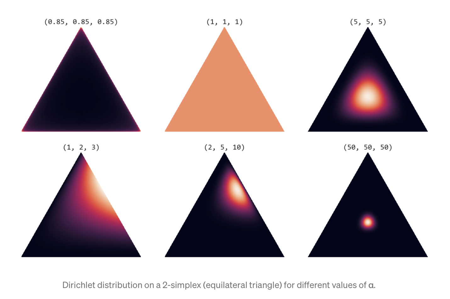
Parameter $\alpha$ governs the shape of the distribution inside the simplex. In particular the sum $\alpha_0 = \sum_{k}\alpha_{k}$ controls the strength of the distribution (how peaked it is). If $\alpha_k < 1$ for all $k$, we get spikes at the corners of the simplex. For values of $\alpha_k > 1$, the distribution tends toward the centre of the simplex. As $\alpha_0$ increases, the distribution becomes more tightly concentrated around the centre of the simplex. [Source: https://towardsdatascience.com/dirichlet-distribution-a82ab942a879]
The normalized form of the Dirichlet distribution is
$$\begin{align} Dir(\mu|\alpha) = \frac{\Gamma(\alpha_0)}{\Gamma(\alpha_1)…\Gamma(\alpha_K)} \prod_{k=1}^{K} \mu_{k}^{\alpha_k - 1} \end{align}$$
where $\Gamma(x)$ is the gamma function and
$$\begin{align} \alpha_{0} = \sum_{k=1}^{K}\alpha_{k} \end{align}$$
The posterior distribution for the parameter ${\mu_k}$ takes the form
$$\begin{align} p(\mu|D,\alpha) \propto p(D|\mu)Dir(\mu|\alpha) \propto \prod_{k=1}^{K} \mu_{k}^{\alpha_k + m_k - 1} \end{align}$$
The normalization coefficient can be obtained by comparion and the final posterior distribution takes the form
$$\begin{align} p(\mu|D,\alpha) = Dir(\mu|\alpha + m) = \frac{\Gamma(\alpha_0+N)}{\Gamma(\alpha_1+m_1)…\Gamma(\alpha_K+m_k)}\prod_{k=1}^{K} \mu_{k}^{\alpha_k + m_k - 1} \end{align}$$
where $m=(m_1,m_2,…,m_K)^T$. The parameter $\alpha_k$ can be interpreted as the effective number of observations of $x_k=1$.