2.3 The Gaussian Distribution
Gaussian Distribution is a widely used model for the distribution of continous variables. For a single variable $x$, the gaussian distribution is given as
$$\begin{align} N(x|\mu,\sigma^2) = \frac{1}{(2\pi\sigma^2)^{1/2}} exp \bigg[\frac{-1}{2\sigma^2} (x-\mu)^2\bigg] \end{align}$$
where $\mu$ and $\sigma^2$ are mean and variance respectively. For a $D$ dimensional vector $X$, the multivariate gaussian distribution takes the form
$$\begin{align} N(X|\mu,\Sigma) = \frac{1}{(2\pi)^{D/2}}\frac{1}{|\Sigma|^{1/2}} exp \bigg[\frac{-1}{2} (X-\mu)^T\Sigma^{-1}(X-\mu)\bigg] \end{align}$$
where $\mu$ is a $D$ dimensional mean vector and $\Sigma$ is a $D\times D$ dimensional covariance matrix with $|\Sigma|$ being its determinant.
One of the major application of Normal/Gaussian distribution is in Central Limit Theorem. It states that the distribution of sample means approximates a gaussian distribution as the sample size gets larger, regardless of the population’s distribution.
Gaussian distribution is functionally dependent on $X$ is through the quadratic form which appears in the exponent shown below.
$$\begin{align} \Delta^2 = (X-\mu)^T\Sigma^{-1}(X-\mu) \end{align}$$
The quantity $\Delta$ is called the Mahalnobis distance from $\mu$ to $X$ which reduces to Euclidean distance when $\Sigma$ is identity matrix. For the surface in $X$-space on which this quadratic form is constant, the gaussian distribution will be constant. Another thing to note is: $\Sigma$ is a real symmetric matrix. Being a real symmetric matrix, its eigenvalues will be real and its eigenvectors will form an orthonormal set. The eigenvector equation can be given as:
$$\begin{align} \Sigma u_i = \lambda_i u_i \end{align}$$
where $u_i$ are eigenvectors with $\lambda_i$ being the corresponding eigenvalues. The condition of orthonormality of eigenvectors give us
$$\begin{align} u_i^Tu_j = I_{ij} \end{align}$$
where $I_{ij} = 1$ $\forall i=j$ and $0$ otherwise. The covariance matrix $\Sigma$ can be represented in terms of eigenvalues and eigenvectors as
$$\begin{align} \Sigma = \sum_{i=1}^{D}\lambda_iu_iu_i^T \end{align}$$
The inverse covaraince matrix $\Sigma^{-1}$ can be expressed as
$$\begin{align} \Sigma^{-1} = \sum_{i=1}^{D}(\lambda_iu_iu_i^T)^{-1} = \sum_{i=1}^{D}\frac{1}{\lambda_i}(u_iu_i^T)^{-1} = \sum_{i=1}^{D}\frac{1}{\lambda_i}u_iu_i^T \end{align}$$
Substituting it into the quadratic form, it reduces to
$$\begin{align} \Delta^2 = (X-\mu)^T \bigg[ \sum_{i=1}^{D} \frac{1}{\lambda_i}u_iu_i^T\bigg] (X-\mu) = \sum_{i=1}^{D} \frac{y_i^2}{\lambda_i} \end{align}$$
The derivation of above expression is shown below.
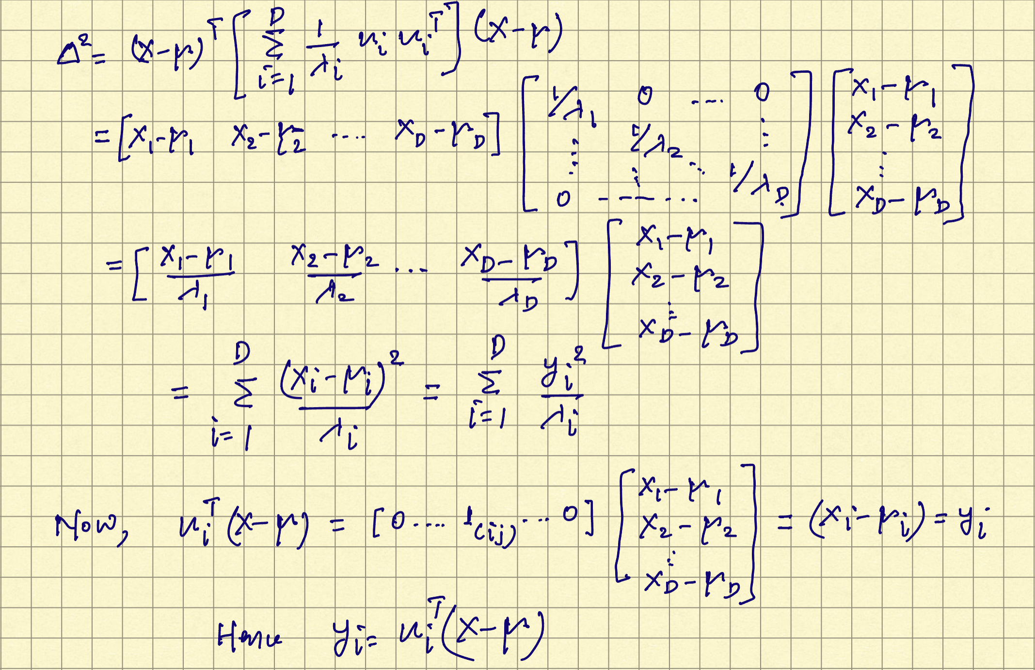
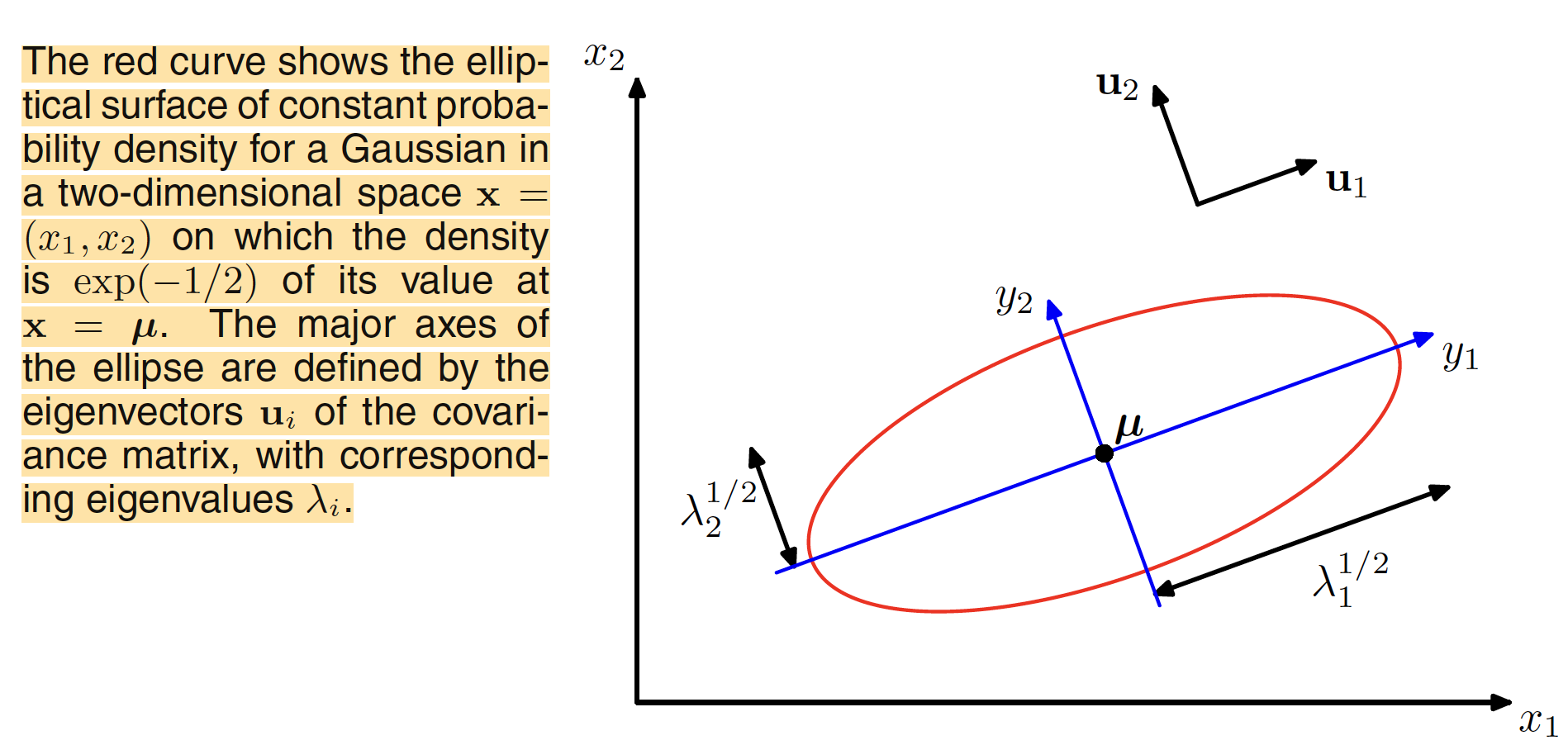
$y_i$ can be interpreted as the original $x_i$ coordinate shifted by mean $\mu_i$ and rotated to align the eigenvector $u_i$. In the new coordinate system, $Y = U(X-\mu)$ where $U$ is the transpose of eigenvector matrix of the covariance matrix and is orthogonal. The representation of rotated gaussina distribution is shown below. If all the eigenvalues $\lambda_i$ are positive, the surface of constant density is an ellipsoid with their centers at $\mu$ and axes along $u_i$. For the Gaussian distribution to be well defined, all the eigenvalues $\lambda_i$ shoulb be positive which makes the covariance matrix positive definite.
Using the eigenvalue decomposition of covariance matrix, its determinant is given as
$$\begin{align} |\Sigma|^{1/2} = \prod_{j=1}^{D}(\lambda_j)^{1/2} \end{align}$$
In the new coordinate system, eigenvectors being orthonormal, the Gaussian distribution takes the form of $D$ independent univariate gaussian distributions.
$$\begin{align} p(Y) = \prod_{j=1}^{D}\frac{1}{(2\pi\lambda_j)^{1/2}} exp\bigg[\frac{-y_j^2}{2\lambda_j}\bigg] \end{align}$$
Expectation of $X$ under the Gaussian distribution can be derived as
$$\begin{align} E[X] = \frac{1}{(2\pi)^{D/2}}\frac{1}{|\Sigma|^{1/2}} \int exp \bigg[\frac{-1}{2} (X-\mu)^T\Sigma^{-1}(X-\mu)\bigg]XdX \end{align}$$
Using $Z=X-\mu$, we get $dX=dZ$ and the expression reduces to
$$\begin{align} E[X] = \frac{1}{(2\pi)^{D/2}}\frac{1}{|\Sigma|^{1/2}} \int exp \bigg[\frac{-1}{2} Z^T\Sigma^{-1}Z\bigg] (Z+\mu)dZ \end{align}$$
$$\begin{align} = \frac{1}{(2\pi)^{D/2}}\frac{1}{|\Sigma|^{1/2}} \bigg(\int exp \bigg[\frac{-1}{2} Z^T\Sigma^{-1}Z\bigg]ZdZ + \int exp \bigg[\frac{-1}{2} Z^T\Sigma^{-1}Z\bigg]\mu dZ\bigg) \end{align}$$
$$\begin{align} = \frac{1}{(2\pi)^{D/2}}\frac{1}{|\Sigma|^{1/2}} \bigg(0 + \int exp \bigg[\frac{-1}{2} Z^T\Sigma^{-1}Z\bigg]\mu dZ\bigg) \end{align}$$
$$\begin{align} = \mu\frac{1}{(2\pi)^{D/2}}\frac{1}{|\Sigma|^{1/2}} \int exp \bigg[\frac{-1}{2} Z^T\Sigma^{-1}Z\bigg] dZ = \mu \end{align}$$
The second order moment of a univariate Gaussian is given as $E[x^2]$. For a multivariate Gaussian, this is defined as $E[XX^T]$ and is computed as
$$\begin{align} E[XX^T] = \frac{1}{(2\pi)^{D/2}}\frac{1}{|\Sigma|^{1/2}} \int exp \bigg[\frac{-1}{2} (X-\mu)^T\Sigma^{-1}(X-\mu)\bigg]XX^TdX \end{align}$$
$$\begin{align} = \frac{1}{(2\pi)^{D/2}}\frac{1}{|\Sigma|^{1/2}} \int exp \bigg[\frac{-1}{2} Z^T\Sigma^{-1}Z\bigg] (Z+\mu)(Z+\mu)^TdZ \end{align}$$
$$\begin{align} = \frac{1}{(2\pi)^{D/2}}\frac{1}{|\Sigma|^{1/2}} \int exp \bigg[\frac{-1}{2} Z^T\Sigma^{-1}Z\bigg] (ZZ^T + \mu Z^T + Z\mu^T + \mu\mu^T)dZ \end{align}$$
The terms with $\mu Z^T,Z\mu^T$ will vanish as the expression inside the integral is an odd function. $\mu\mu^T$ being constant, the integral for the expression having it will be $\mu\mu^T$ (as the Gaussian distribution is normalized). The integral of the term with $ZZ^T$ will come out to be $\Sigma$. Hence,
$$\begin{align} E[XX^T] = \mu\mu^T + \Sigma \end{align}$$
This gives us the covariance as
$$\begin{align} Cov[X] = \Sigma \end{align}$$
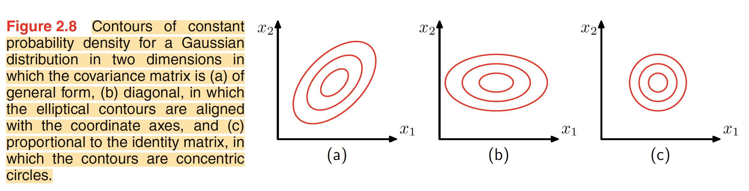
Total number of independent parameters in a multivariate Gaussian will depend on the dimension $D$ of the dataset. We will have a total of $D$ independet parameters in mean $\mu$. For the covariance matrix $\Sigma$, we will have a total of ${D \choose 2} = \frac{D(D+1)}{2}$ independent parameters. Hence, in the problem of density estimation, we have to come with an estimation of a total of $\frac{D(D+3)}{2}$ parameters. Using restrictive form of covariance matrix reduces the number of independent parameters drastically. For a diagonal covariance matrix, we will have a total of $2D$ parameters to estimate with the contours of constant density as axis-aligned ellipsoids. If we further restrict the covariance matrix to be proportional to identity matrix, we will have a total of $D+1$ independent parameters for estimation and we will get the spherical surface of constant density. The shape of desities for these $3$ cases is shown in the figure below. Restricting the covariance matrix makes the calculation simplified but but it limits the number of degree of freedom in the distribution and hence limits its ability to capture interesting correlation in the dataset.