One goal of pattern recognition is to model the probability distribution $p(x)$ of a random variable $x$ given the finite set of points $x_1, x_2, …, x_N$. This problem is known as density estimation. For simplicity, we can assume that the points are independent and identically distributed. There can be infinitely many distributions that can give rise to the given data points with any distribution that is non-zero at the points $x_1, x_2, …, x_N$ as a potential candidate.
A parametric distribution is the distribution which is governed by a set of parameters. For example, a gaussian distribution is governed by its mean and variance. Hence, to model a distribution, we need a procedure for determining the suitable values for these parameters. There are two ways to do it: Frequentist and Bayesian approach. In a frequentist approach, we determine the values of parameters by optimizing some criteria like the likelihood function, i.e. we have to find a parameter set $w$ which will maximize the probability of observing the given data points $D$, $p(D|w)$. In a Bayesian setting, we assume some prior distribution over the parameters and then use Bayes’ theorem to compute the corresponding posterior distribution given the observed data points $D$. If we assume that the posterior distribution takes the same form as prior, the analysis for Bayesian approach will be greatly simplified.
One major limitation of parametric approach is that we assume a specific functional form of the distribution, which may turn out to be inappropriate for a particular application. An alternative approach is given by a nonparametric density estimation methods where the form of the distribution depends on the size of the dataset and it’s parameter usually controls the model complexity.
2.1 Binary Variables
Let us consider a simple coin flip experiment where we have the set of outcomes defined as $x = {0,1}$, with $x=1$ represnting heads and $x=0$ representing tails. The probability of $x=1$ will be denoted by a parameter $\mu$ where $0 \leq \mu \leq 1$ as:
$$\begin{align} p(x=1|\mu) = \mu \end{align}$$
This gives us the probability of $x=0$ as $p(x=0|\mu) = 1-\mu$. The probability distribution over $x$ can be given as:
$$\begin{align} Bern(x|\mu) = \mu^x(1-\mu)^{1-x} \end{align}$$
and is called as Bernoulli Distribution. The distribution is normalized and its mean and variance are given as:
$$\begin{align} E[x] = \mu; Var[x] = \mu(1 - \mu) \end{align}$$
For a dataset $D = {x_1, x_2, …, x_N}$, assuming the the points are drawn independently from $p(x|\mu)$, the likelihood function $p(D|\mu)$ can be defined as:
$$\begin{align} p(D|\mu) = \prod_{n=1}^{N} p(x_n|\mu) = \prod_{n=1}^{N}\mu^{x_n}(1-\mu)^{1-x_n} \end{align}$$
In a frequentist setting, we can estimate the value of parameter $\mu$ by maximizing the likelihood function $p(D|\mu)$ or maximizing the log of the likelihood function instead. For Bernoulli distribution, the log likelihood function is given as:
$$\begin{align} \ln p(D|\mu) = \sum_{n=1}^{N} \ln p(x_n|\mu) = \sum_{n=1}^{N} [x_n \ln \mu + (1-x_n)\ln (1 - \mu)] \end{align}$$
The maximum likelihood estimator of $\mu$ can be determined by setting the derivative of $\ln p(D|\mu)$ with respect to $\mu$ equal to zero and is derived as:
$$\begin{align} \frac{\delta\ln p(D|\mu)}{\delta\mu} = \sum_{n=1}^{N} \bigg[\frac{x_n}{\mu} - \frac{(1-x_n)}{(1 - \mu)}\bigg] = 0 \end{align}$$
$$\begin{align} \implies \sum_{n=1}^{N} \bigg[(1 - \mu)x_n - \mu(1-x_n)\bigg] = 0 \end{align}$$
$$\begin{align} \implies \sum_{n=1}^{N} \bigg[x_n - \mu\bigg] = 0 \end{align}$$
$$\begin{align} \implies \mu_{ML} = \frac{1}{N}\sum_{n=1}^{N} x_n \end{align}$$
which is the sample mean. If the number of observations with $x=1$ is $m$, the the MLE estimator of the parameter $\mu$ is given as:
$$\begin{align} \mu_{ML} = \frac{m}{N} \end{align}$$
One of the major darwaback of the frequentist approach is lets say we just have $5$ data points and for all those data points, the outcome is head, i.e. $m=5,N=5$. This means that the maximum likelihood estimator of mean is $\mu_{ML} = \frac{5}{5} = 1$. Hence the maximum likelihood estimator will predict that all the future outcomes will be head. This is an extreme example of overfitting associated with maximum likelihood estimator.
Another important distribution is Binomial Distribution. It is the distribution for the number of observations for which $x=1$ given that we have a total of $N$ data points (number of heads in $N$ coin tosses). Binomial distribution is given as:
$$\begin{align} Bin(m|N,\mu) = {N \choose m} \mu^m (1-\mu)^{N-m} \end{align}$$
where
$$\begin{align} {N \choose m} = \frac{N!}{m!(N-m)!} \end{align}$$
$m=x_1+x_2+…+x_N$ where $x_i$ is a bernoulli variable. For independent events, the mean and variance of sum is the sum of the means and variances. Hence,
$$\begin{align} E[m] = N\mu \end{align}$$
$$\begin{align} Var[m] = N\mu(1-\mu) \end{align}$$
2.1.1 Beta Distribution
As explained above, frequentist approach can lead to highly overfitted results in some of the cases (mainly when the size of dataset is samll). In order to treat the problem with the Bayesian approach, we need to define a prior probability $p(\mu)$ over the parameter $\mu$. As posterior probability is the product of prior and the likelihood function and likelihood function takes the form of product of factors $\mu^x(1-\mu)^{1-x}$, if we choose a prior to be proportional to the powers of $\mu$ and $1-\mu$, the posterior distribution will have the same functional form. This property is called conjugacy and the prior and posterior distributions are called conjugate distributions with prior distribution being conjugate prior of the likelihood function. Beta Distribution has this property and is given as:
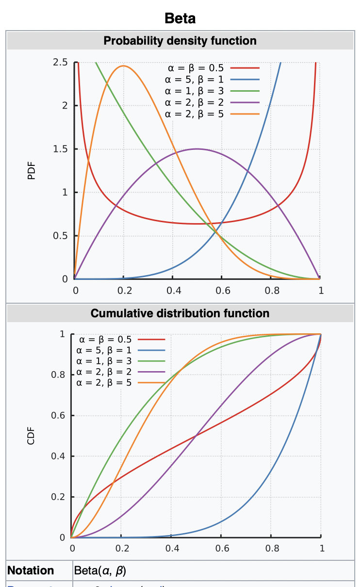
$$\begin{align} Beta(\mu|a,b) = \frac{\Gamma(a+b)}{\Gamma(a)\Gamma(b)} \mu^{a-1}(1-\mu)^{b-1} \end{align}$$
where $\Gamma(x)$ is the gamma function defined as:
$$\begin{align} \Gamma(x) = \int_{0}^{\infty} u^{x-1}e^{-u}du \end{align}$$
Beta distribution is normalized with its mean and variance given as:
$$\begin{align} E[\mu] = \frac{a}{a+b} \end{align}$$
$$\begin{align} Var[\mu] = \frac{ab}{(a+b)^2(a+b+1)} \end{align}$$
The parameters $a,b$ are hyperparameters as they control the distribution of parameter $\mu$. The PDF and CDF of Beta distribution is shown below with $a,b$ denoted as $\alpha, \beta$ respectively.
For a binomial likelihood function where $l=N-m$, the posterior distribution with beta prior is given as:
$$\begin{align} Beta(\mu|m,l,a,b) \propto \mu^{m+a-1}(1-\mu)^{l+b-1} \end{align}$$
The posterior distribution has the same functional form as the prior and hence beta distribution maintains the property of conjugate prior with respect to likelihood function. The normalization coefficient of posterior distribution can be obtained by comparing it with prior and which gives the posterior distribution as:
$$\begin{align} Beta(\mu|m,l,a,b) = \frac{\Gamma(m+a+l+b)}{\Gamma(m+a)\Gamma(l+b)} \mu^{m+a-1}(1-\mu)^{l+b-1} \end{align}$$
The effect of observing $m$ observations of $x=1$ and $l$ observations of $x=0$ is the increase in the value of $a$ by $m$ and that of $b$ by $l$. The hyperparametrs $a,b$ can be simply interpreted as the effective number of observations of $x=1$ and $x=0$. This means that the posterior distribution can act like prior if we observe additional data. Hence, we can take observations one at a time and can update the posterior distribution by updating the parameters and normalizing constant. This sequential approach of learning is one of the key property of Bayesian method. This sequential approach is independent of choice of prior and likelihood function and depends only on the assumption of i.i.d. data.
Let us say that our goal is to predict the outcome of the next trial based on the evidence that we have. This means we have to evaluate $p(x=1|D)$ which takes the form
$$\begin{align} p(x=1|D) = \int_{0}^{1} p(x=1|\mu)p(\mu|D)d\mu = \int_{0}^{1} \mu p(\mu|D)d\mu = E[\mu|D] \end{align}$$
Using the mean of beta distribution, we get
$$\begin{align} p(x=1|D) = \frac{m+a}{m+a+l+b} \end{align}$$
If we have infinitely large dataset (i.e. $m,l \to \infty$), above quantity reduces to the maximum likelihood estimate $a/(a+b)$. As the number of data point increases, the distribution becomes sharply peaked with variance decreasing. For $a,b \to \infty$, the variance $Var[\mu] = \frac{ab}{(a+b)^2(a+b+1)} \to 0$. This is a general property of Bayesian learning. As we observe more and more data, the uncertaininty in posterior distribution will steadily decrease.