1.6 Information Theory
Some amount of information is recieved when we observe the value of a discrete random variable $x$. If a highly improbable event has occured, the amount of information received is higher. For an event which was certain to happen, no amount of information is received. Hence, the measure of information $h(x)$ will therefore depend on the probability distribution $p(x)$ and will be a monotnic function of $p(x)$. For two unrelated events $x$ and $y$, the information gain from observing both of them $h(x,y) = h(x) + h(y)$ is sum of the information gained from each of them separately. From probability prespective, the joint probability of unrelated event is given as $p(x,y) = p(x)p(y)$. Hence, the information gain will be a logarithmic function of $p(x)$ and can be denoted as:
$$\begin{align} h(x) = -\log_{2}p(x) \end{align}$$
The entropy of a random variable $x$ is the average information gained over the probability distribution $p(x)$ and is given as:
$$\begin{align} H[x] = \sum_{x}p(x)h(x) = -\sum_{x}p(x)\log_{2}p(x) \end{align}$$
Entropy can also be viewed as the average amount of information transmitted when we transmit the value of random variable. For example, for a random variable $x$ having $8$ possible states, each of which is equally likely, the entropy is given as:
$$\begin{align} H[x] = -\sum_{x}p(x)\log_{2}p(x) = -8 \times \frac{1}{8}\log_{2}\frac{1}{8} = 3 \end{align}$$
This means that in order to communicate the value of $x$, we need to transmit a message of $3$ bits. It can easily be observed that a nonuniform distribution has a smaller entropy than a uniform one. The noiseless coding theorem states that the entropy is a lower bound on the number of bits needed to transmit the state of a random variable.
Entropy can also be viewed as a measure of disorder. Consider a set of $N$ identical objects that are to be divided amongst a set of bins, such that there are $n_i$ objects in $i^{th}$ bin. Total number of ways it can be done is called the multiplicity and is given as:
$$\begin{align} W = \frac{N!}{\prod_{i}n_i!} \end{align}$$
The entropy is then defined as the logarithm of multiplicity sacled by an appropriate constant.
$$\begin{align} H = \frac{1}{N}\ln W = \frac{1}{N} = \frac{1}{N} \ln N! - \frac{1}{N} \sum_{i} \ln n_i! \end{align}$$
As $N \to \infty$, $\ln N! \simeq N \ln N - N$ and the expresion reduces to
$$\begin{align} H = - \lim_{N \to \infty} \sum_{i} \bigg(\frac{n_i}{N}\bigg)\ln \bigg(\frac{n_i}{N}\bigg) = - \lim_{N \to \infty} \sum_{i} p_i \ln p_i \end{align}$$
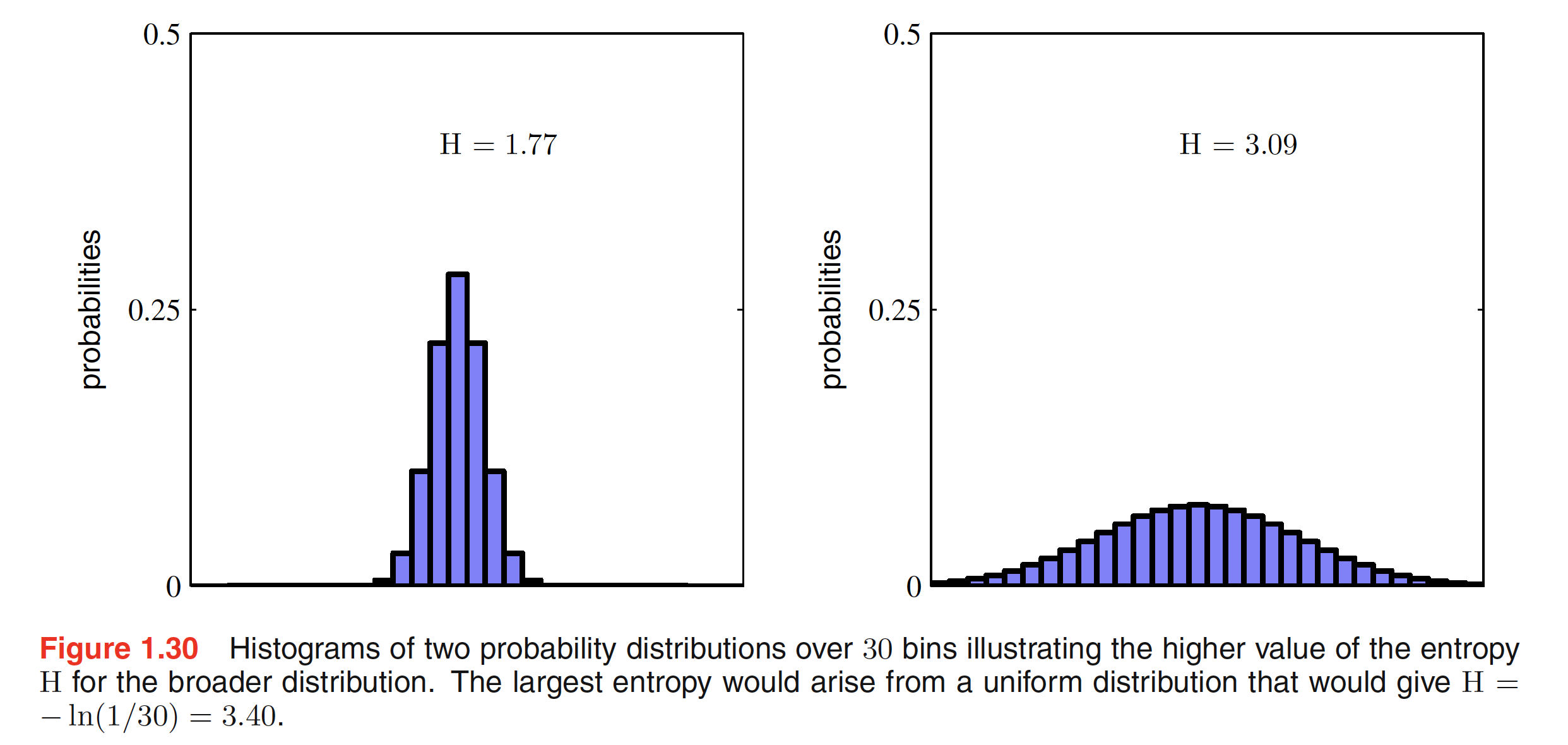
where $p_i = \lim_{N \to \infty}(n_i/N)$ is the probability of an object being assigned to the $i^{th}$ bin. As we saw earlier that more uniform a distribution is, higher the entropy. Hence, for distributions $p(x_i)$ that are sharply peaked around few values will have a relatively low entrpy compared to more evenly spread distributions. This phenomenon is shown in the below figure.
Finding the maximum entropy is a maximization problem with a constraint. The problem can be stated as: maximize $H = -\sum_{i} p(x_i) \ln p(x_i)$ subjected to the constraint $\sum_{i}p(x_i) = 1$. The constraint can be enforced using Lagrange Multiplier and reduces to:
$$\begin{align} \tilde{H} = -\sum_{i} p(x_i) \ln p(x_i) + \lambda\bigg(\sum_{i}p(x_i) - 1\bigg) \end{align}$$
The solution to this optimization problem is $p(x_i) = 1/M$ $\forall i$, with a correspnding value of entropy as $H = \ln M$.
Differential Entropy, also reffered as Continous Entropy is a measure of average surprisal of a random variable to continous probability distribution. One of the main concern with the continuous random variables is that their values typically have 0 probability, and therefore would require an infinite number of bits to encode. Hence instead of measuring the absolute entropy, we measure the relative entropy.
1.6.1 Relative Entropy and Mutual Information
Consider some unknown distribition $p(x)$ which is modeled as approximating distribution $q(x)$. If we use $q(x)$ to encode $x$, the average additional amount of information needed to encode $x$ is given as:
$$\begin{align} KL(p||q) = - \int p(x) \ln q(x) + \int p(x) \ln p(x) = - \int p(x) ln \bigg(\frac{q(x)}{p(x)}\bigg) \end{align}$$
This is known as the relative entropy or Kulback-Leibler Divergence between the distributions $p(x)$ and $q(x)$. It should be noted that $KL(p||q) \neq KL(q||p)$. Kullback-Leibler divergence satisfies $KL(p||q) \geq 0$ with equality holding when $p(x) = q(x)$.
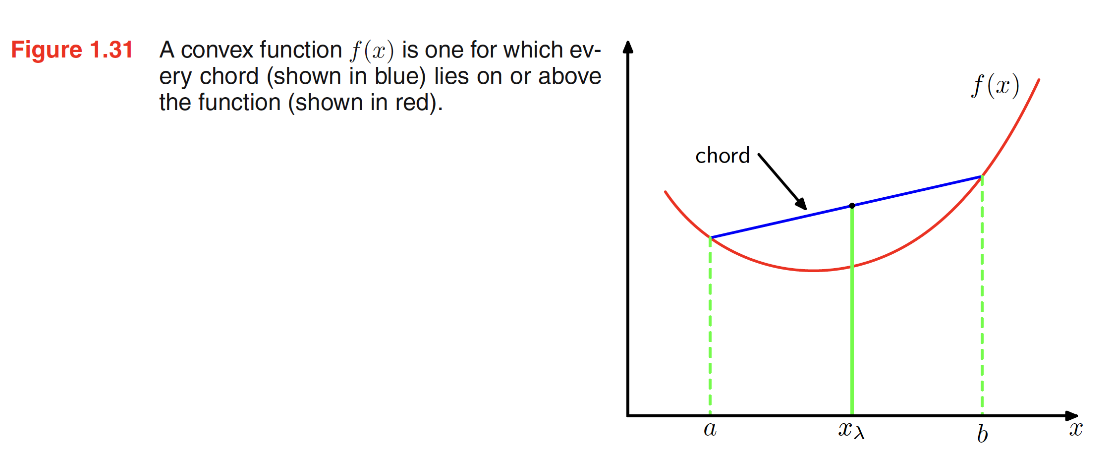
Convex Functions are the functions for which every chord lies on or above the function. For a function $f(x)$ to be convex, $f(\lambda a + (1-\lambda)b) \leq \lambda f(a) + (1 - \lambda)f(b)$. This can easily be viewed by considerig the property that any point in between two points $m$ and $n$ can be represented as $\lambda m + (1-\lambda)n$ where $0 \leq \lambda \leq 1$. A convex function is shown in the figure below. Convexity also implies that the second derivative of the function is positive everywhere.
In general, a convex function satisfies
$$\begin{align} f\bigg( \sum_{i=1}^{M} \lambda_i x_i \bigg) \leq \sum_{i=1}^{M} \lambda_i f(x_i) \end{align}$$
where $\lambda_i \geq 0$ and $\sum_{i=1}\lambda_i = 1$. Above inequality is called as Jensen’s Inequality. If $\lambda_i$ is interpreted as the probability distribution for a discrete variable $x$ taking the values ${x_i}$, then Jensen’s Inequality can be written as:
$$\begin{align} f(E[x]) \leq E[f(x)] \end{align}$$
For continuous variable, Jenesen’s Inequality takes the form
$$\begin{align} f\bigg(\int xp(x) dx\bigg) \leq \int f(x)p(x) dx \end{align}$$
As $-\ln x$ is a convex function and $\int q(x) dx = 1$, applying Jenesen’s inequality to KL-divergence, we get
$$\begin{align} KL(p||q) = - \int p(x) ln \bigg(\frac{q(x)}{p(x)}\bigg)dx \geq - ln\bigg( \int \frac{q(x)}{p(x)} p(x) dx\bigg) = - ln\bigg( \int q(x) dx\bigg) = 0 \end{align}$$
There is an intimate relationship between data compression and density estimation as the most efficient compression is achieved when we know the true distribution. If we use a distribution that is different from the true one, then we must necessarily have a less efficient coding, and on average the additional information that must be transmitted is (at least) equal to the Kullback-Leibler divergence between the two distributions. Let’s say an unknown distribution $p(x)$ is modeled using $q(x|\theta)$ where $\theta$ is a set of adjustable parameters. One way to determine the parameter $\theta$ is to minimize the KL-divergence between $p(x)$ and $q(x|\theta)$ with respect to $\theta$. In this setting $p(x)$ is unknown but as we have observed $N$ points from the distribution, the KL-divergence can be approximated as (integral replaced with summation):
$$\begin{align} KL(p||q) \simeq \sum_{i=1}^{N} [-\ln q(x_i|\theta) + \ln p(x_i)]p(x_i) \end{align}$$
The second term is independet of $\theta$ and we can even ignore $p(x_i)$ while doing the maximization with respect to $\theta$. The first term $\ln q(x_i|\theta)$ is the log likelihood function for $\theta$ under the distribution $q(x|\theta)$. Hence minimizing KL-divergence is equivalent to maximizing the likelihood function.