1.5 Decision Theory
The idea behind decision theorey is to convert the model probabilities (mainly for classification problem) to a decision. Given an input vector $x$ with the corresponding output $t$, the joint probability distribution $p(x,t)$ will provide the complete summary of uncertainity associated with these variables. Determination of $p(x,t)$ from the training data is a difficult problem and hence in a practical setting, we are more intersted in taking decisions based on probable value of $t$ for a given $x$. This intution sets the premise for the decision theory.
Let us consider an example of a medical diagnosis problem where given an X-ray image ($x$), we have to predict whether the patient has the cancer (class $C_1$) or not (class $C_2$), i.e. we are interested in the probabilities $p(C_k|x)$. Using Bayes’ Theorem, these probabilities can be expressed as:
$$\begin{align} p(C_k | x) = \frac{p(x|C_k)p(C_k)}{p(x)} \end{align}$$
$p(C_k)$ can be interpreted as the prior probabilities of the classes and $p(C_k | x)$ is the probability post-evidence. If our aim is to minimize the chance of assigning $x$ to the wrong class, then we should choose the class having highest posterior probability.
1.5.1 Minimizing the Misclassification Rate
The goal of minimum misclassification can be achieved by dividing the entire input space into regions $R_k$ called as decision regions, one for each class, such that all the points in $R_k$ will be assigned to $C_k$. The boundaries between the decision regions are called as decision boundaries. For a two class case, a mistake occurs if a point belonging to class $C_1$ is assigned to class $C_2$ or vice versa. The probability of mistake is given as:
$$\begin{align} p(mistake) = p(x \in R_1, C_2) + p(x \in R_2, C_1) = \int_{R_1} p(x,C_2)dx + \int_{R_2} p(x,C_1)dx \end{align}$$
Hence, to minimize the probability of mistake, if $p(x, C_1) > p(x, C_2)$ for a given value of $x$, then we should assign that $x$ to class $C_1$. As $p(x, C_k) = p(C_k|x)p(x)$, and the term $p(x)$ is common for all the classes, the minimum probability of mistake is obtained if each value of $x$ is assigned to the calss for which the posterior probability $p(C_k|x)$ is largest.
For a generic case of $K$ classes, it is easier to maximize the probability of being correct which is given as:
$$\begin{align} p(correct) = \sum_{k=1}^{K} p(x \in R_k, C_k) = \sum_{k=1}^{K} \int_{R_k} p(x,C_k)dx \end{align}$$
which is maximized when the regions $R_k$ are chosen such that each $x$ is assigned to the class for which $p(x,C_k)$ or $p(C_k|x)$ is maximum.
1.5.2 Minimizing the Expected Loss
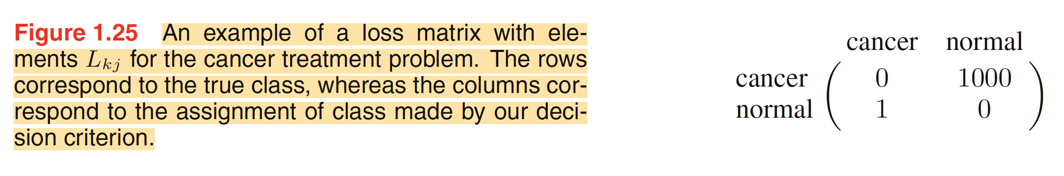
Loss function or Cost function is a single overall measure of loss incurred in taking any of the available decisions or actions. Our goal is then to minimize the total loss incurred. Instead, we can even maximize the Utility function. We can encode loss function (or the level of loss incurred when a decison is taken) as a matrix $L$ whose entry $L_{kj}$ is the loss incurred when a new value $x$ belonging to the true class $C_k$ is assigned to class $C_j$ (where $j$ may or may not be $k$). A typical loss matrix for the cancer classification problem is shown below.
The optimal solution for any decision problem is the one which minimizes the loss function. But, the loss function depends on the true class which is unknown. We can however represent the uncertainity in true class by the joint probability $p(x,C_k)$ for any input $x$ and hence we can minimize the average loss instead. This average is computed with respect to the distribution of $p(x,C_k)$ and is given as:
$$\begin{align} E[L] = \sum_{k}\sum_{j}\int_{R_j}L_{kj}p(x,C_k)dx \end{align}$$
Hence, our goal is to choose the region $R_j$ such that for each $x$, $\sum_{k}L_{kj}p(x,C_k)$ is minimized. Replacing $p(x,C_k)$ with $p(C_k|x)p(x)$, we have minimize $\sum_{k}L_{kj}p(C_k|x)$ instead. This can be done easily as we know each of the posterior probabilities.
1.5.3 The Reject Option
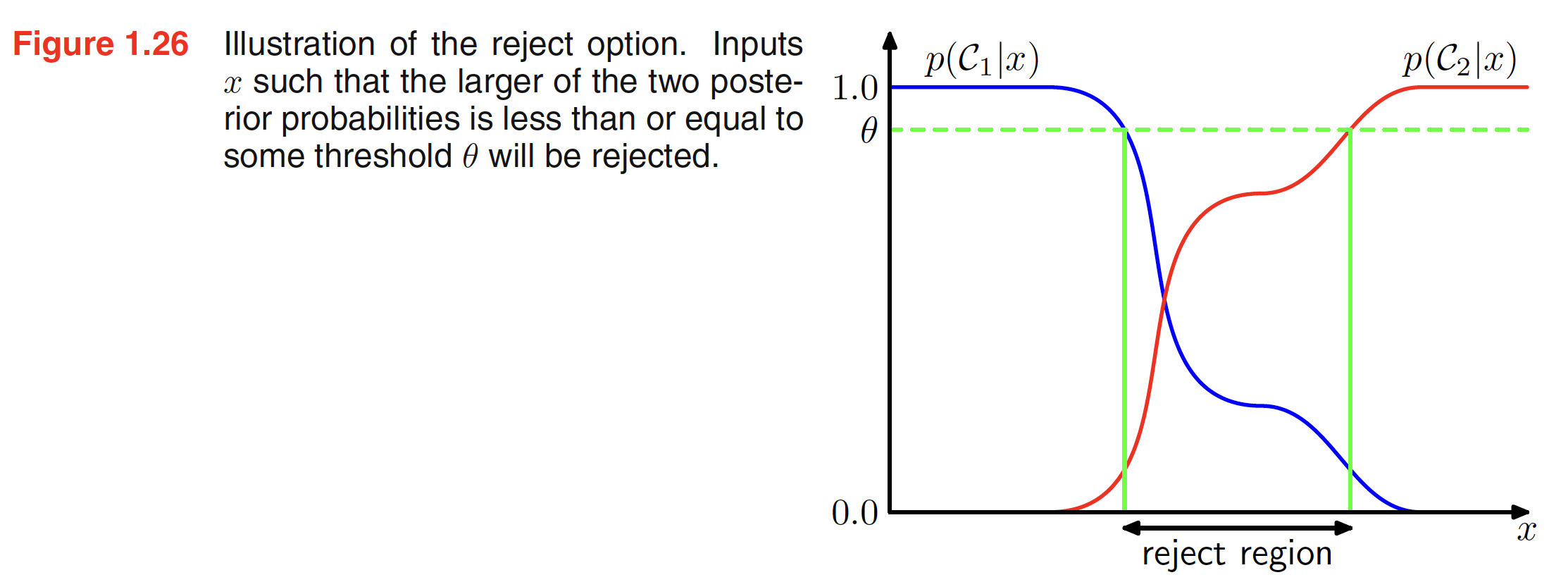
Classification errors mainly arise from the regions of input space where posterior probability $p(C_k|x)$ is significantly less than unity or equivalently the joint distributions $p(x,C_k)$ are comparable. These are the regions where we are uncertain about the classification and hence it will be better avoid making decisions on them. This is known as the reject option. We can achieve this by selecting a threshold $\theta$ and rejecting the inputs $x$ for which the largest of the posterior probabilities $p(C_k|x) \leq \theta$. The illustration of reject region is shown below.
1.5.4 Inference and Decision
The classification problem can be broken down into two stages: inference stage in which a training data is used to learn the model for $p(C_k|x)$ and decision satge where these posterior probabilities are used to make class assignments. An alternate will be to club these stages together and simply learn a function (discriminant function) that maps the input $x$ directly to the decision.
Hence, any classification problem can be soved using three approaches. The approaches in their decreasing order of complexity are as follows.
-
In approach one, we implicitly or explicitly model the distribution of inputs as well as outputs $p(x,C_k)$. These models are called as generative models as they can be used to generate sythetic data points in the input space. Directly modeling the distribution is the most difficult problem to solve.
-
Another approach is to model $p(C_k|x)$ and then used decision theory to assign each new $x$ to one of the classes. Approaches that model the posterior probability directly are called as discriminative models.
-
The third approach is to find a function $f$ (called as discriminant function) which directly maps the input $x$ to the output class.
One of the drawbacks of last approach is the fact that we cannot combine different models together if we directly model for discriminant functions. Lets say that in the cancer detection problem, we have the access to the blood data (denoted as $x_B$ and X-ray image denoted as $x_I$) of individuals as well. From the second approach, if we want to generate a combined model, we can easily club the two individual model posterior probabilities together to find the combined model posterior probability.
$$\begin{align} p(C_k|x_I,x_B) \propto p(x_I,x_B|C_k)p(C_k) \end{align}$$
Assuming that the blood data and X-ray image are independent, we have
$$\begin{align} p(x_I,x_B|C_k)p(C_k) = p(x_I|C_k)p(x_B|C_k) \end{align}$$
Hence,
$$\begin{align} p(C_k|x_I,x_B) \propto p(x_I|C_k)p(x_B|C_k)p(C_k) = \frac{p(C_k|x_I)p(C_k|x_B)}{p(C_k)} \end{align}$$
1.5.5 Loss function for Regression
In a regression problem, the decision state consists of choosing an estimate $y(x)$ of the value of $t$ for a given input $X$. Suppose, in doinf so we incur a loss $L(t, y(x))$. The expected loss is given as:
$$\begin{align} E[L] = \int\int L(t, y(x))p(x,t)dx \ dt \end{align}$$
A common choice is squared loss given as $L(t, y(x)) = [y(x) - t]^2$. In this case, the expected loss can be written as
$$\begin{align} E[L] = \int\int [y(x) - t]^2 p(x,t)dx \ dt \end{align}$$
Our goal is to choose $y(x)$ which will minimize $E[L]$.
$$\begin{align} \frac{\delta E[L]}{\delta y(x)} = 2\int [y(x) - t] p(x,t) dt = 0 \end{align}$$
Solving for $y(x)$, we get
$$\begin{align} y(x) = \frac{\int tp(x,t)dt}{\int p(x,t)dt} = \frac{\int tp(x,t)dt}{p(x)} = \int t\frac{p(x,t)}{p(x)}dt = \int tp(t|x)dt = E_{t}[t|x] \end{align}$$
The three approaches to solve the regression problem in decreasing order of complexity are as follows.
-
First solve the inference problem to get the joint density $p(x,t)$. Normalize this to find the conditional density $p(t|x)$ and then marginalize it to find the conditional mean $E_t[t|x]$.
-
In the second approach we directly model $p(t|x)$ and then marginalize it to find the conditional mean $E_t[t|x]$
-
Lastly, we can directly model the regression function $y(x)$ from the training data.
Instead of squared loss, we can even use lower or higher order loss, called as Minkowski Loss whose expectation is given as:
$$\begin{align} E[L_q] = \int\int |y(x) - t|^q p(x,t)dx \ dt \end{align}$$