1.2 Probability Theory
Consider two random variables $X,Y$ where $X$ can take any of the values $x_i$ where $i=1,2,…,M$ and $Y$ can take the values $y_j$ where $j=1,2,…,L$. In a total of $N$ trials, both $X,Y$ are sampled and the number of trials for which $X=x_i,Y=y_j$ is $n_{ij}$. The number of trials in which $X=x_i$ is $c_i$ and $Y=y_j$ is $r_j$ respectively. Then, the joint probability of $X$ taking the value $x_i$ and $Y$ taking the value $y_j$ is given as:
$$\begin{align} p(X=x_i,Y=y_j) = \frac{n_{ij}}{N} \end{align}$$
The marginal probability of $X$ taking the value $x_i$ irrespective of the value of $Y$ is given as:
$$\begin{align} p(X=x_i) = \frac{c_{i}}{N} = \sum_{j=1}^{L}p(X=x_i,Y=y_j) \end{align}$$
where $c_i = \sum_{j}n_{ij}$. This is also called as the sum rule of probability. For $X=x_i$, the fraction of instances for which $Y=y_j$ is called as conditional probability of $Y=y_j$ given $X=x_i$ and is given as:
$$\begin{align} p(Y=y_j|X=x_i) = \frac{n_{ij}}{c_{i}} = \frac{p(X=x_i,Y=y_j)}{p(X=x_i)} \end{align}$$
This relation is also called as produt rule of probability. We can simply denote the joint and marginal probability as $p(X,Y)$(probability of $X$ and $Y$) and $p(Y|X)$ (probability of $Y$ given $X$). The Bayes’ Rule of probability is given as:
$$\begin{align} p(Y|X) = \frac{p(X|Y)p(Y)}{p(X)} \end{align}$$
where the denominator is:
$$\begin{align} p(X) = \sum_{Y}p(X|Y)p(Y) \end{align}$$
$X$ and $Y$ are said to be independent if $p(X,Y) = p(X)p(Y)$. Prior probability expresses the probability before some evidence is taken into account. Posterior probability expresses the probability after some evidence is taken into account.
1.2.1 Probability Desnities
For continuous variables, probability can be computed using probability densities. If the probability of a real-valued variable $x$ falling in the range $(x, x+\delta x)$ is given as $p(x)\delta x$ for $\delta x \to 0$, then $p(x)$ is called the probability density over $x$. The probability that $x$ will lie in the interval $(a,b)$ is given as:
$$\begin{align} p(x \in (a,b)) = \int_{a}^{b}p(x)dx \end{align}$$
It should be noted that $p(x) \geq 0$ and $\int_{-\infty}^{\infty}p(x)dx = 1$. Let there be a change of variable $x = g(y)$ where the probability density functions are $p_x(x)$ and $p_y(y)$ with $p_x(x) \simeq p_y(y)$. Hence,
$$\begin{align} p_y(y) = p_x(x)\left| \frac{dx}{dy} \right| = p_x(g(y))\left| g^{’}(y) \right| \end{align}$$
For any continuos variable $x$, the probability that it lies in the interval $(\infty, z)$ is given by cumulative distribution function which is defined as
$$\begin{align} P(z) = \int_{-\infty}^{z}p(x)dx \end{align}$$
and satisfies $P^{’}(x) = p(x)$. For the continuous case, the sum and product rule takes the form
$$\begin{align} p(x) = \int p(x,y)dy \end{align}$$
$$\begin{align} p(y|x) = \frac{p(x,y)}{p(x)} \end{align}$$
When $x$ is discrete, $p(x)$ is called as probability mass function.
1.2.2 Expectations and Covariances
Average value of any function $f(x)$ under a probability distribution $p(x)$ is called as the Expectation of $f(x)$ and is denoted as $E[f]$. For discrete distribution, it is given as:
$$\begin{align} E[f] = \sum_{x}f(x)p(x) \end{align}$$
For continuous distribution, it is given as:
$$\begin{align} E[f] = \int f(x)p(x)dx \end{align}$$
For $N$ finite points drawn from a continuous distribution, the expectation can be estimated as:
$$\begin{align} E[f] \simeq \frac{1}{N} \sum_{n=1}^{N} f(x_n) \end{align}$$
For a function of two variables $f(x,y)$, the average of the function with respect to the distribution of $x$ is denoted as $E_{x}[f(x,y)]$. Variance of $f(x)$ is defined as:
$$\begin{align} var[f] = E[(f(x) - E[f(x)])^2] = E[f(x)^2] - E[f(x)]^2 \end{align}$$
which defines how much variability is there in $f(x)$ around its mean value $E[f(x)]$. In the case of two vectors of random variables $x$ and $y$, the covariance is a matrix defined as
$$\begin{align} cov[x,y] = E_{x,y}[(x-E[x])(y^T - E[y^T])] = E_{x,y}[xy^T] - E[x]E[y^T] \end{align}$$
It should be noted that $cov[x] = cov[x,x]$.
1.2.3 Bayesian Probabilities
Bayes’ Theorem can be used to convert prior probability to posterior probability by incorporating the evidence provided by the observed data. We can adopt this approach when making inferences about the quantities such as parameters $\mathbf{w}$ in the polynomial curve fitting example. We can encode our assumption about $\mathbf{w}$ as its prior distribution $p(\mathbf{w})$ befor observing the data. The distribution of observed data $D= (t_1, t_2, …, t_n)$ given prior $\mathbf{w}$ is encoded as $p(D|\mathbf{w})$. Then, Bayes’ Theorem can be used to derive the posterior distribution $p(\mathbf{w}|D)$ as
$$\begin{align} p(\mathbf{w}|D) = \frac{p(D|\mathbf{w})p(\mathbf{w})}{p(D)} \end{align}$$
$p(D|\mathbf{w})$ is expresses how probable the observed data $D$ is for different settings of the parameter vector $\mathbf{w}$. It is called as the likelihood function. The denominator $p(D)$ can be computed as $p(D) = \int p(D|\mathbf{w})p(\mathbf{w})d\mathbf{w}$.
In a frequentist setting, a widely used estimator is a maximum likelihood estimator. In maximum likelihood estimator, $\mathbf{w}$ is set to a value which maximizes the likelihood function $p(D|\mathbf{w})$. The negative log of the likelihood function is called as the error function. As negative logarithm is monotonically decreasing, maximizing the likelihood is equivalent to minimizing the error function.
In a Bayesian setting, we choose prior distributions $p(\mathbf{w})$ and $p(D|\mathbf{w})$, which are then used to compute the posterior distributions $p(\mathbf{w}|D)$. One criticisim of this approach is that these prior distributions are often chosen as per the mathematical convenience rather than as a reflection of prior beliefs. Reducing the dependence on prior is one motive for noninformative priors which may lead to better results.
1.2.4 The Gaussian Distribution
For a real-valued variable $x$, the gaussian or normal distribution is defined as:
$$\begin{align} N(x|\mu,\sigma^2) = \frac{1}{(2\pi\sigma^2)^{1/2}}exp\left\{{\frac{-1}{2\sigma^2}(x-\mu)^2}\right\} \end{align}$$
where $\mu$ is the mean and $\sigma^2$ being variance ($\sigma$ being standard deviation). Reciprocal of the variance $\beta = \frac{1}{\sigma^2}$ is called as precision. Being a probability distribution, it satisfies following properties.
$$\begin{align} N(x|\mu,\sigma^2) > 0 \end{align}$$
$$\begin{align} \int_{-\infty}^{\infty}N(x|\mu,\sigma^2)dx = 1 \end{align}$$
The mean and variance of the gaussian distribution can be calculated as:
$$\begin{align} E[x] = \int_{-\infty}^{\infty}N(x|\mu,\sigma^2)xdx = \mu \end{align}$$
$$\begin{align} E[x^2] = \int_{-\infty}^{\infty}N(x|\mu,\sigma^2)x^2dx = \mu^2 + \sigma^2 \end{align}$$
$$\begin{align} var[x] = E[x^2] - E[x]^2 = \sigma^2 \end{align}$$
Let us suppose we want to determine the parameters of a gaussian distribution ($\mu, \sigma^2$) based on $N$ points drawn from it. Let these observations are $\mathbf{x} = (x_1, x_2, …, x_N)^T$ where they are drawn independenty from the same gaussian distribution (called as independent and identically distributed). As they are independent, we can write
$$\begin{align} p(\mathbf{x}|\mu,\sigma^2) = \prod_{n=1}^{N}N(x_n|\mu,\sigma^2) \end{align}$$
This is the likelihood function of a gaussian distribution. The goal is to find the values of parematers $\mu$ and $\sigma^2$ which maximize this likelihood function. Instead of maximizing the likelihood function, we can maximize the log of it.
$$\begin{align} ln(p(\mathbf{x}|\mu,\sigma^2)) = \sum_{n=1}^{N}ln[N(x_n|\mu,\sigma^2)] \end{align}$$
$$\begin{align} = \frac{-1}{2\sigma^2}\sum_{n=1}^{N}(x_n - \mu)^2 - \frac{N}{2}ln(2\pi) - \frac{N}{2}ln(\sigma^2) \end{align}$$
Taking derivative with respect to $\mu$ and equating it to $0$, we get
$$\begin{align} \mu_{ML} = \frac{1}{N}\sum_{n=1}^{N}x_n \end{align}$$
which is the sample mean. Taking the derivative with respect to $\sigma^2$ and equating it to 0, we get
$$\begin{align} \sigma^2_{ML} = \frac{1}{N}\sum_{n=1}^{N}(x_n - \mu_{ML})^2 \end{align}$$
which is the sample variance measured w.r.t. the sample mean. Maximum likelihood estimators for mean and varince are functions of data set values $x_1, x_2, …, x_n$. Considering the expectations of these quantities with respect to the data set values, we get
$$\begin{align} E[\mu_{ML}] = \mu \end{align}$$
$$\begin{align} E[\sigma^2_{ML}] = \left(\frac{N-1}{N}\right)\sigma^2 \end{align}$$
Hence, maximum likelihood estimator will underestimate the true variance by a factor of $\frac{N-1}{N}$. The unbiased estimate of variance is
$$\begin{align} \tilde{\sigma}^2 = \left(\frac{N}{N-1}\right)\sigma^2_{ML} = \frac{1}{N-1}\sum_{n=1}^{N}(x_n - \mu_{ML})^2 \end{align}$$
1.2.5 Curve fitting re-visited
The curve fitting example can be seen as deriving a polynomial function $y(x,\mathbf{w})$ which has parameters $\mathbf{w}$ and input $x$. The predicted value $y(x,\mathbf{w})$ should be as close as possible to the target $t$. We can assume that for a given value of $x$, the corresponding value of $t$ follows a gaussian distribution with mean $y(x,\mathbf{w})$ and variance $\sigma^2$ (or precision $\beta = \frac{1}{\sigma^2}$). This is depicted in the below figure.
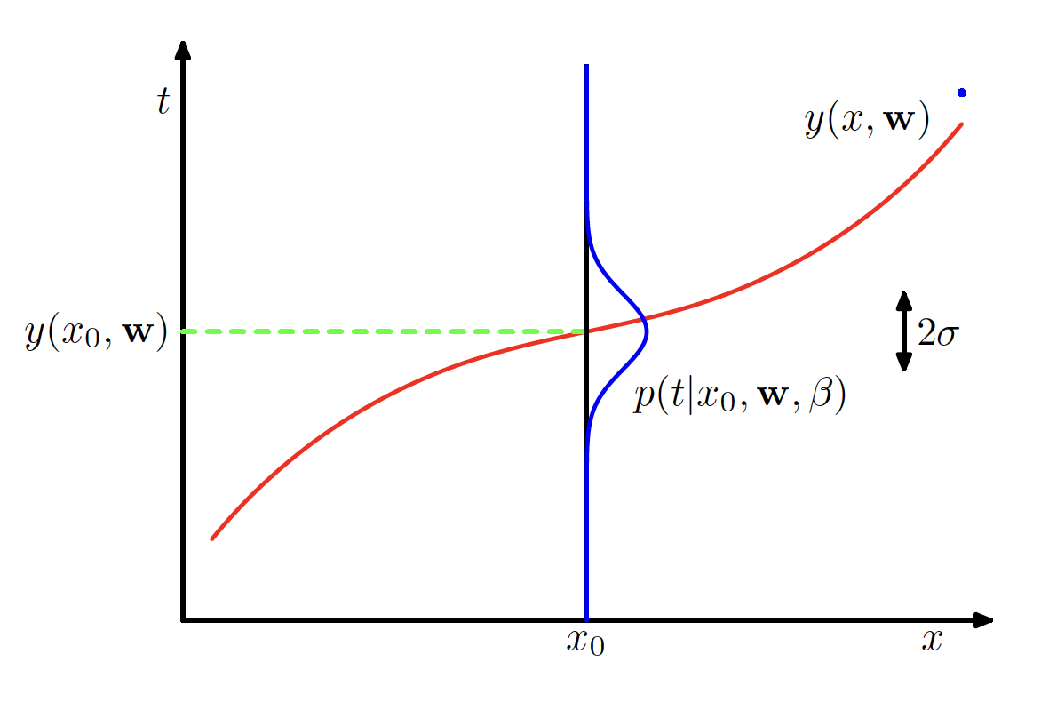
Hence, we have
$$\begin{align} p(t | x, \mathbf{w}, \beta) = N(t|y(x,\mathbf{w}),\beta^{-1}) \end{align}$$
We have to maximize the likelihood for the entire training dataset $\mathbf{{x,t}}$, which is $p(\mathbf{t | x}, \mathbf{w}, \beta)$ to get the value of $\mathbf{w}$ and $\beta$. If we assume that the data is drawn independently from the distribution, the maximum likelihood function is given as
$$\begin{align} p(\mathbf{t|x}, \mathbf{w}, \beta) = \prod_{n=1}^{N}N(t_n|y(x_n,\mathbf{w}),\beta^{-1}) \end{align}$$
Taking the logarithm, we get
$$\begin{align} ln(p(\mathbf{t|x}, \mathbf{w}, \beta)) = \frac{-\beta}{2}\sum_{n=1}^{N}{y(x_n,\mathbf{w}) - t_n}^2 - \frac{N}{2}ln(2\pi) + \frac{N}{2}ln(\beta) \end{align}$$
The maximum likelihood estimator of the polynomial coefficient $\mathbf{w}$ deonted as $\mathbf{w_{ML}}$ is obtained by maximizing the log likelihood with respect to $\mathbf{w}$. As the last two terms $- \frac{N}{2}ln(2\pi) + \frac{N}{2}ln(\beta)$ does not depend on $\mathbf{w}$, we can omit them, i.e. we simply have to maximize $\frac{-\beta}{2}\sum_{n=1}^{N}{y(x_n,\mathbf{w}) - t_n}^2$ w.r.t. $\mathbf{w}$. $\beta$ being a constant, we can remove it and by reversing the sign, we have to minimize $\frac{1}{2}\sum_{n=1}^{N}{y(x_n,\mathbf{w}) - t_n}^2$, which is the sum of squares error fucntion. Hence, the sum-of-squares error function has arisen as a consequence of maximizing likelihood under the assumption of a Gaussian noise distribution. Maximizing w.r.t. $\beta$, we get
$$\begin{align} \beta_{ML} = \frac{1}{N}\sum_{n=1}^{N}\{y(x_n,\mathbf{w_{ML}}) - t_n\}^2 \end{align}$$
Using the bayseian approach, we can even get the error in predictio of $t$ as we get the predictive distribution over $t$ instead of just a point estimate. The predictive distribution is given as
$$\begin{align} p(t | x, \mathbf{w_{ML}}, \beta_{ML}) = N(t|y(x,\mathbf{w_{ML}}),\beta^{-1}_{ML}) \end{align}$$
If we further include the prior distribution of $\mathbf{w}$ and assume that it follows a gaussian distribution with mean $0$ and precision $\alpha$. As we know that the multivaraite gaussian for a $D$ dimensional vector is given as
$$\begin{align} N(\mathbf{x|\mu,\Sigma}) = \frac{1}{(2\pi)^{D/2}} \frac{1}{|\mathbf{\Sigma}|^{1/2}} exp\left\{{\frac{-1}{2}(\mathbf{x-\mu})^T}\mathbf{\Sigma}^{-1}(\mathbf{x-\mu})\right\} \end{align}$$
where $\mathbf{x,\mu}$ are $D$ dimensional vectors and $\mathbf{\Sigma}$ is a $D \times D$ covariance matrix. The covariance matrix for the distribution of $\mathbf{w}$ can be represented as $\mathbf{\Sigma} = \alpha^{-1}\mathbf{I}$, where $\mathbf{I}$ is a $(M+1) \times (M+1)$ matrix, which gives us $|\mathbf{\Sigma}| = \frac{1}{\alpha^{M+1}}$. Hence, we get
$$\begin{align} p(\mathbf{w}|\alpha) = N(\mathbf{w} |0,\alpha^{-1}\mathbf{I}) = \left(\frac{\alpha}{2\pi}\right)^{(M+1)/2} exp\left\{{\frac{-\alpha}{2}\mathbf{w}^T}\mathbf{w}\right\} \end{align}$$
Using Bayes’ Theorem, we have
$$\begin{align} p(\mathbf{w|x,t},\alpha,\beta) \propto p(\mathbf{t|x,w},\beta) p(\mathbf{w}| \alpha) \end{align}$$
We can now maximize the posterior distribution of $\mathbf{w}$ by taking the logarithm and following the similar process and we can eventually reach at the conclusion that we have to minimze the following term instead
$$\begin{align} \frac{\beta}{2} \sum_{n=1}^{N}{y(x_n,\mathbf{w}) - t_n}^2 + \frac{\alpha}{2}\mathbf{w}^T\mathbf{w} \end{align}$$
Hence, maximizing the posterior distribution is equivalent to minimizing the regularized sum-of-squares error function.