Any pattren recognition or machine learning task can be primarily divided into two categories: Supervised and Unsupervised Learning. In a supervised machine learning problem, we have the input and corresponding desired output. For any supervised learning problem, the aim of the pattern recognition algorithm is to come up with an algorithm or model which can predict the output given the input. Based on the output, the supervised learning problem can be divided into two categories: Classification (when we have a finite number of discrete output) and Regression (if the desired output consists of one or more continuous variables). For an unsupervised learning problem, we don’t have the desired output for the input variables. The goal of pattern recognition is: to discover groups of similar examples within the data (clustering), to determine the distribution of data within the input space (density estimation), to project the data from a high-dimensional space to low-dimensional space etc..
Let us take an example of a supervised pattern recognition problem.
1.1 Polynomial Curve Fitting
For simplicity, we can generate the data for this task from the function $Sin(2\pi x)$ with random gaussian noise included in the targetv varible, i.e, for any input $x$, target $t=Sin(2\pi x) + \epsilon$. Let the training set consists of $N$ samples with inputs as $\mathbf{x} = (x_1, x_2, …, x_N)^T$ and the corresponding target variables as $\mathbf{t} = (t_1, t_2, …, t_N)^T$. Let the polynomial fuction used for the prediction, whose order is $M$, is:
$$\begin{align} y(x,\mathbf{w}) = w_0 + w_1x + w_2x^2 + … + w_Mx^M = \sum_{j=0}^{M}w_jx^j \end{align}$$
This polynomial function is linear with respect to the coefficients $w$. The goal of the pattern recognition task is to minimize the error in predicting $t$. Or we can say that we have to minimize some error function which should encode how much we deviated from the actual value while doing the prediction. One of the common choice of error fuction is:
$$\begin{align} E(\mathbf{w}) = \frac{1}{2}\sum_{n=1}^{N}[y(x_n,\mathbf{w}) - t_n]^2 \end{align}$$
The error function is quadratic in $w$ and hence taking it’s derivative w.r.t $w$ and equating it to $0$ gives us a unique solution $w^{*}$ for the problem.
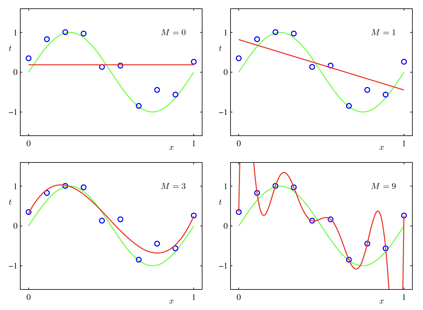
One of the important parameter in deciding how well the solution will perform on the unseen data is the order of the polynomial function $M$. As shown in the below figure, if we keep on increasing $M$, we will get a perfect fit on the training data getting the training error $E(w^{*}) = 0$ (called as overfitting) but the prediction on unseen data will be flawed. The best fit polynomial seems to be the one which has on order $M=3$.
One of the insights which we can get after looking at the coefficients $w^{*}$ obtained from polynomial of various degrees. As $M$ increases, the magnitude of the coefficient gets large.
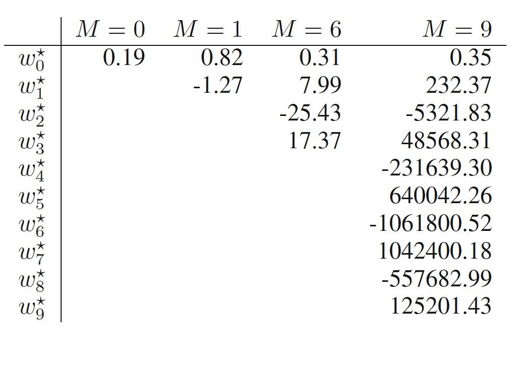
Based on these coefficients, one of the techniques which can be used to coompensate for the problem of overfitting is regularization which involves adding a penalty term to the error function which discourages the coefficients from getting larger in magnitude. The modified error functio is given as:
$$\begin{align} \widetilde{E}(\mathbf{w}) = \frac{1}{2}\sum_{n=1}^{N}(y(x_n,\mathbf{w}) - t_n)^2 + \frac{\lambda}{2}\left\Vert w \right\Vert^2 \end{align}$$
where $\left\Vert w \right\Vert^2 = w^Tw = w_0^2 + w_1^2 + … + w_M^2$. This technique is also called as shrinkage method and a quadratic regularizer is called as ridge regression.
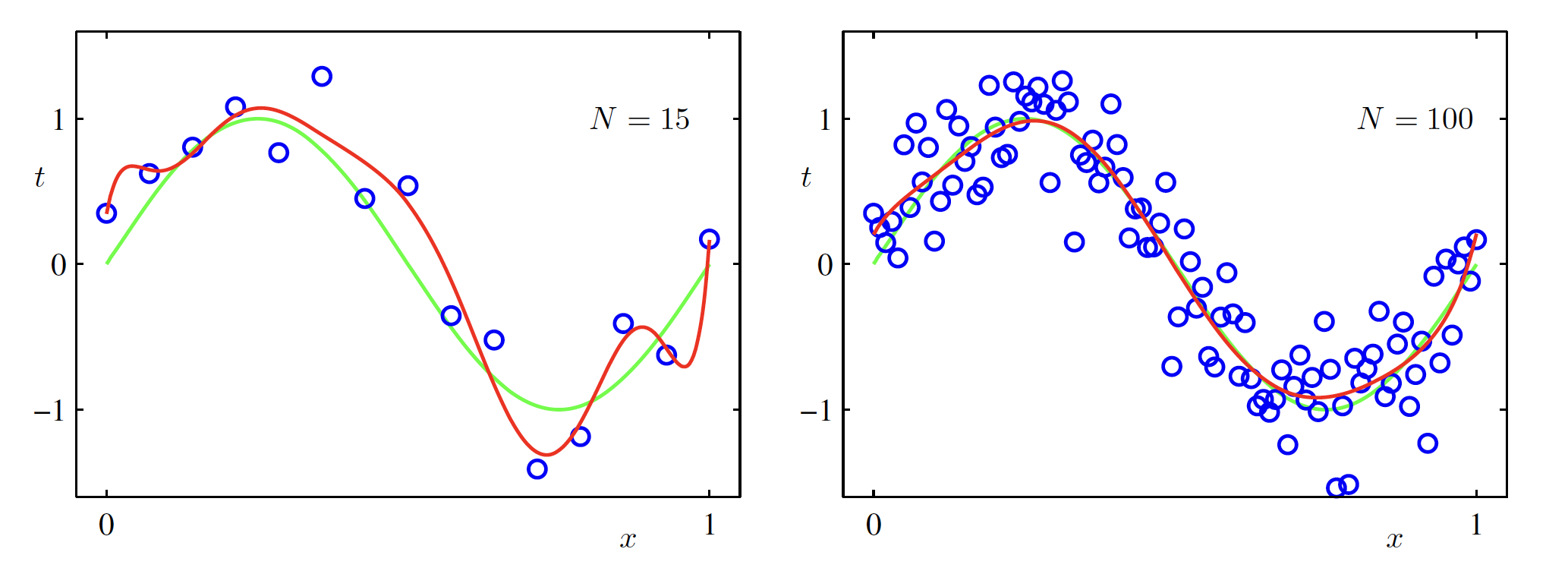
Another way to reduce overfitting or to use the complex models for prediction is by increasing the sample size of the training data. The same order $M=9$ polynomial is fit on $N=15$ and $N=100$ datapoints and result is shown in the left and the right figure below. It can be seen that the increasing the number of datapoinsts reduces the problem of overfitting.