ISLR Chapter 7: Moving Beyond Linearity (Part 6: Exercises

Applied

Q6. In this exercise, you will further analyze the Wage data set considered throughout this chapter.

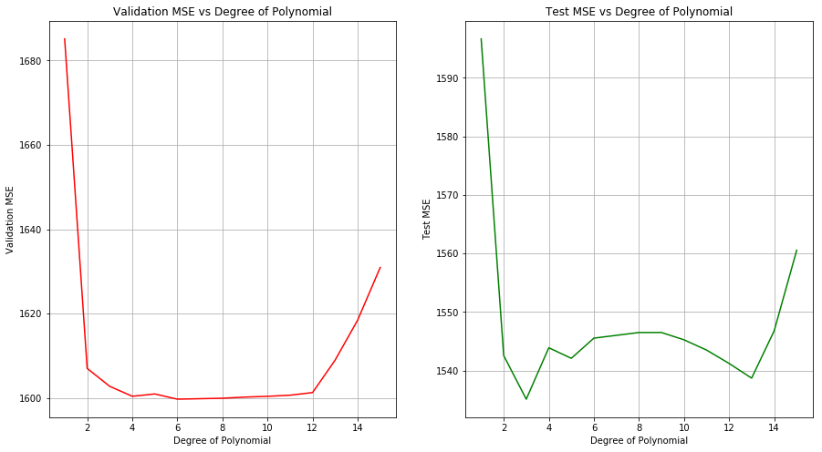
(a) Perform polynomial regression to predict wage using age. Use cross-validation to select the optimal degree d for the polynomial. What degree was chosen, and how does this compare to the results of hypothesis testing using ANOVA? Make a plot of the resulting polynomial fit to the data.

Sol: The optimal degree of polynomial selected from cross-validation is 4. From the ANOVA of models of degree 1 to 5, it is found that the models of degree 2 and 3 are significant. The test MSE shows the lowest value for degree 3 model as well.

import pandas as pd
import numpy as np

wage = pd.read_csv("data/Wage.csv")
wage.head()

	Unnamed: 0	year	age	sex	maritl	race	education	region	jobclass	health	health_ins	logwage	wage
0	231655	2006	18	1. Male	1. Never Married	1. White	1. < HS Grad	2. Middle Atlantic	1. Industrial	1. <=Good	2. No	4.318063	75.043154
1	86582	2004	24	1. Male	1. Never Married	1. White	4. College Grad	2. Middle Atlantic	2. Information	2. >=Very Good	2. No	4.255273	70.476020
2	161300	2003	45	1. Male	2. Married	1. White	3. Some College	2. Middle Atlantic	1. Industrial	1. <=Good	1. Yes	4.875061	130.982177
3	155159	2003	43	1. Male	2. Married	3. Asian	4. College Grad	2. Middle Atlantic	2. Information	2. >=Very Good	1. Yes	5.041393	154.685293
4	11443	2005	50	1. Male	4. Divorced	1. White	2. HS Grad	2. Middle Atlantic	2. Information	1. <=Good	1. Yes	4.318063	75.043154

from sklearn import preprocessing
from sklearn.model_selection import LeaveOneOut
from sklearn.model_selection import train_test_split
from sklearn.linear_model import LinearRegression
from sklearn.metrics import mean_squared_error

np.random.seed(5)

def polynomial_regression(X_train, Y_train, X_test, Y_test, M):
    validation_MSE = {}
    test_MSE = {}

    for m in M:
        poly = preprocessing.PolynomialFeatures(degree=m)
        X_ = poly.fit_transform(X_train)

        mse = 0
        loo = LeaveOneOut() # Leave one out cross-validation
        for train_index, test_index in loo.split(X_):
            X, X_CV = X_[train_index], X_[test_index]
            Y, Y_CV = Y_train[train_index], Y_train[test_index]
            # Linear Regression (including higher order predictors)
            model = LinearRegression(fit_intercept=True)
            model.fit(X, Y)
            p = model.predict(X_CV)
            mse += mean_squared_error(p, Y_CV)
        validation_MSE[m] = mse/len(X_)

        # Compute test MSE for the model
        model = LinearRegression(fit_intercept=True)
        model.fit(X_, Y_train)
        p = model.predict(poly.fit_transform(X_test))
        test_MSE[m] = mean_squared_error(p, Y_test)

    # Plot validation MSE
    lists = sorted(validation_MSE.items()) # sorted by key, return a list of tuples
    x, y = zip(*lists) # unpack a list of pairs into two tuples
    fig = plt.figure(figsize=(15, 8))
    ax = fig.add_subplot(121)
    plt.plot(x, y, color='r')
    plt.grid()
    ax.set_xlabel('Degree of Polynomial')
    ax.set_ylabel('Validation MSE')
    ax.set_title('Validation MSE vs Degree of Polynomial')

    lists = sorted(test_MSE.items()) # sorted by key, return a list of tuples
    x, y = zip(*lists) # unpack a list of pairs into two tuples
    ax = fig.add_subplot(122)
    plt.plot(x, y, color='g')
    plt.grid()
    ax.set_xlabel('Degree of Polynomial')
    ax.set_ylabel('Test MSE')
    ax.set_title('Test MSE vs Degree of Polynomial')
    plt.show()


X_train, X_test, y_train, y_test = train_test_split(wage[['age']], wage[['wage']], test_size=0.1)
polynomial_regression(X_train, y_train.values, X_test, y_test, [1,2,3,4,5,6,8,9,10,11,12,13,14,15])

import statsmodels.api as sm

poly = preprocessing.PolynomialFeatures(degree=1)
X_ = poly.fit_transform(wage[['age']])
model1 = sm.OLS(wage[['wage']], X_)
model1 = model1.fit()

poly = preprocessing.PolynomialFeatures(degree=2)
X_ = poly.fit_transform(wage[['age']])
model2 = sm.OLS(wage[['wage']], X_)
model2 = model2.fit()

poly = preprocessing.PolynomialFeatures(degree=3)
X_ = poly.fit_transform(wage[['age']])
model3 = sm.OLS(wage[['wage']], X_)
model3 = model3.fit()

poly = preprocessing.PolynomialFeatures(degree=4)
X_ = poly.fit_transform(wage[['age']])
model4 = sm.OLS(wage[['wage']], X_)
model4 = model4.fit()

poly = preprocessing.PolynomialFeatures(degree=5)
X_ = poly.fit_transform(wage[['age']])
model5 = sm.OLS(wage[['wage']], X_)
model5 = model5.fit()

sm.stats.anova_lm(model1, model2, model3, model4, model5)

/Users/amitrajan/Desktop/PythonVirtualEnv/Python3_VirtualEnv/lib/python3.6/site-packages/scipy/stats/_distn_infrastructure.py:879: RuntimeWarning: invalid value encountered in greater
  return (self.a < x) & (x < self.b)
/Users/amitrajan/Desktop/PythonVirtualEnv/Python3_VirtualEnv/lib/python3.6/site-packages/scipy/stats/_distn_infrastructure.py:879: RuntimeWarning: invalid value encountered in less
  return (self.a < x) & (x < self.b)
/Users/amitrajan/Desktop/PythonVirtualEnv/Python3_VirtualEnv/lib/python3.6/site-packages/scipy/stats/_distn_infrastructure.py:1821: RuntimeWarning: invalid value encountered in less_equal
  cond2 = cond0 & (x <= self.a)

	df_resid	ssr	df_diff	ss_diff	F	Pr(>F)
0	2998.0	5.022216e+06	0.0	NaN	NaN	NaN
1	2997.0	4.793430e+06	1.0	228786.010128	143.593107	2.363850e-32
2	2996.0	4.777674e+06	1.0	15755.693664	9.888756	1.679202e-03
3	2995.0	4.771604e+06	1.0	6070.152124	3.809813	5.104620e-02
4	2994.0	4.770322e+06	1.0	1282.563017	0.804976	3.696820e-01

(b) Fit a step function to predict wage using age, and perform crossvalidation to choose the optimal number of cuts. Make a plot of the fit obtained. Code Source: https://rpubs.com/ppaquay/65563

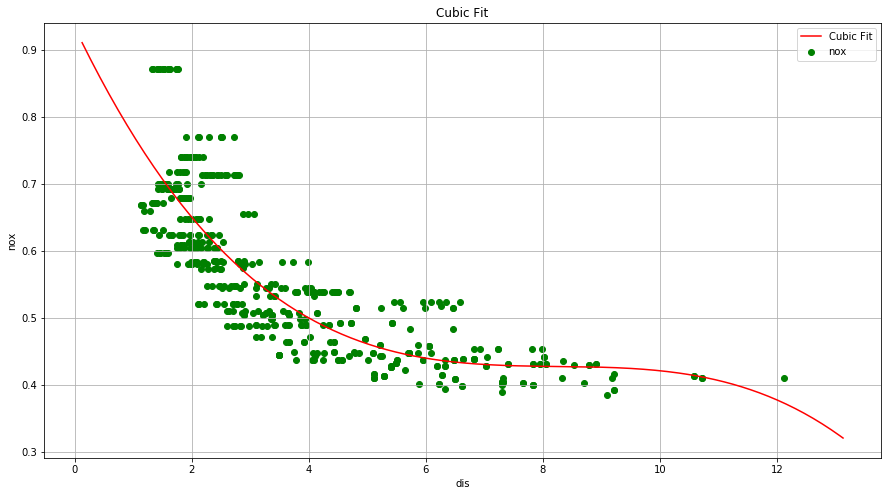
Q9. This question uses the variables dis (the weighted mean of distances to five Boston employment centers) and nox (nitrogen oxides concentration in parts per 10 million) from the Boston data. We will treat dis as the predictor and nox as the response.

(a) Use the poly() function to fit a cubic polynomial regression to predict nox using dis. Report the regression output, and plot the resulting data and polynomial fits.

boston = pd.read_csv("data/Boston.csv")
boston.dropna(inplace=True)

poly = preprocessing.PolynomialFeatures(degree=3)
X_ = poly.fit_transform(boston[['dis']])
model = sm.OLS(boston[['nox']], X_)
result = model.fit()
print(result.summary())

                            OLS Regression Results
==============================================================================
Dep. Variable:                    nox   R-squared:                       0.715
Model:                            OLS   Adj. R-squared:                  0.713
Method:                 Least Squares   F-statistic:                     419.3
Date:                Thu, 20 Sep 2018   Prob (F-statistic):          2.71e-136
Time:                        19:22:18   Log-Likelihood:                 690.44
No. Observations:                 506   AIC:                            -1373.
Df Residuals:                     502   BIC:                            -1356.
Df Model:                           3
Covariance Type:            nonrobust
==============================================================================
                 coef    std err          t      P>|t|      [0.025      0.975]
------------------------------------------------------------------------------
const          0.9341      0.021     45.110      0.000       0.893       0.975
x1            -0.1821      0.015    -12.389      0.000      -0.211      -0.153
x2             0.0219      0.003      7.476      0.000       0.016       0.028
x3            -0.0009      0.000     -5.124      0.000      -0.001      -0.001
==============================================================================
Omnibus:                       64.176   Durbin-Watson:                   0.286
Prob(Omnibus):                  0.000   Jarque-Bera (JB):               87.386
Skew:                           0.917   Prob(JB):                     1.06e-19
Kurtosis:                       3.886   Cond. No.                     2.10e+03
==============================================================================

Warnings:
[1] Standard Errors assume that the covariance matrix of the errors is correctly specified.
[2] The condition number is large, 2.1e+03. This might indicate that there are
strong multicollinearity or other numerical problems.

x = np.linspace(boston['dis'].min()-1, boston['dis'].max()+1, 256, endpoint = True)
y = result.params.const + result.params.x1*x + result.params.x2*(x**2) + result.params.x3*(x**3)

fig = plt.figure(figsize=(15, 8))
plt.plot(x, y, 'red', label="Cubic Fit")
plt.scatter(boston['dis'], boston['nox'], alpha=1, color='green')

plt.xlabel('dis')
plt.ylabel('nox')
plt.title('Cubic Fit')
plt.legend(loc='best')

plt.grid()
plt.show()

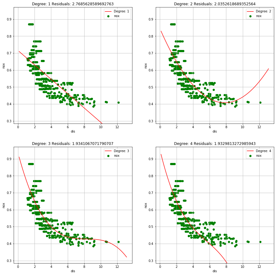
(b) Plot the polynomial fits for a range of different polynomial degrees (say, from 1 to 10), and report the associated residual sum of squares.

def add_polt(ax, x, y, RSS, degree):
    ax.plot(x, y, 'red', label="Degree: " +str(degree))
    ax.scatter(boston['dis'], boston['nox'], alpha=1, color='green')
    ax.set_ylim(boston['nox'].min()-0.1, boston['nox'].max()+0.1)
    ax.set_xlabel('dis')
    ax.set_ylabel('nox')
    ax.set_title('Degree: ' +str(degree) + ' Residuals: ' + str(RSS))
    ax.legend(loc='best')
    ax.grid()

fig = plt.figure(figsize=(15, 40))
x = np.linspace(boston['dis'].min()-1, boston['dis'].max()+1, 256, endpoint = True)

degree = 1
poly = preprocessing.PolynomialFeatures(degree=degree)
X_ = poly.fit_transform(boston[['dis']])
model = sm.OLS(boston[['nox']], X_)
result = model.fit()
y = result.params.const + result.params.x1*x
ax = fig.add_subplot(5, 2, degree)
add_polt(ax, x, y, result.ssr, degree)

degree = 2
poly = preprocessing.PolynomialFeatures(degree=degree)
X_ = poly.fit_transform(boston[['dis']])
model = sm.OLS(boston[['nox']], X_)
result = model.fit()
y = result.params.const + result.params.x1*x + result.params.x2*(x**2)
ax = fig.add_subplot(5, 2, degree)
add_polt(ax, x, y, result.ssr, degree)

degree = 3
poly = preprocessing.PolynomialFeatures(degree=degree)
X_ = poly.fit_transform(boston[['dis']])
model = sm.OLS(boston[['nox']], X_)
result = model.fit()
y = result.params.const + result.params.x1*x + result.params.x2*(x**2) + result.params.x3*(x**3)
ax = fig.add_subplot(5, 2, degree)
add_polt(ax, x, y, result.ssr, degree)

degree = 4
poly = preprocessing.PolynomialFeatures(degree=degree)
X_ = poly.fit_transform(boston[['dis']])
model = sm.OLS(boston[['nox']], X_)
result = model.fit()
y = result.params.const + result.params.x1*x + result.params.x2*(x**2) + result.params.x3*(x**3)
+ result.params.x4*(x**4)
ax = fig.add_subplot(5, 2, degree)
add_polt(ax, x, y, result.ssr, degree)

plt.show()

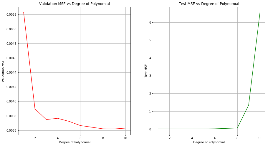
(c) Perform cross-validation or another approach to select the optimal degree for the polynomial, and explain your results.

Sol: The optimal degree of polynomial is 8. Achieved test MSE at this value is decent as well.

np.random.seed(5)
X_train, X_test, y_train, y_test = train_test_split(boston[['dis']], boston[['nox']], test_size=0.2)
polynomial_regression(X_train, y_train.values, X_test, y_test, [1,2,3,4,5,6,8,9,10])

(d) Use the bs() function to fit a regression spline to predict nox using dis. Report the output for the fit using four degrees of freedom. How did you choose the knots? Plot the resulting fit.

(e) Now fit a regression spline for a range of degrees of freedom, and plot the resulting fits and report the resulting RSS. Describe the results obtained.

(f) Perform cross-validation or another approach in order to select the best degrees of freedom for a regression spline on this data. Describe your results.

Q10. This question relates to the College data set.

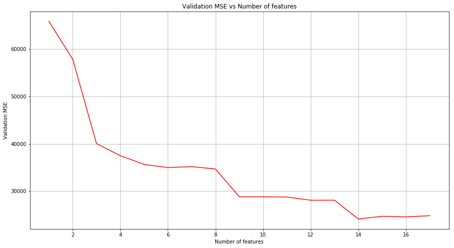
(a) Split the data into a training set and a test set. Using out-of-state-tuition as the response and the other variables as the predictors, perform forward stepwise selection on the training set in order to identify a satisfactory model that uses just a subset of the predictors.

college = pd.read_csv("data/College.csv")
college = college.rename(columns={'Unnamed: 0': 'Name'})
college['Private'] = college['Private'].map({'Yes': 1, 'No': 0})
college.head()

	Name	Private	Apps	Accept	Enroll	Top10perc	Top25perc	F.Undergrad	P.Undergrad	Outstate	Room.Board	Books	Personal	PhD	Terminal	S.F.Ratio	perc.alumni	Expend	Grad.Rate
0	Abilene Christian University	1	1660	1232	721	23	52	2885	537	7440	3300	450	2200	70	78	18.1	12	7041	60
1	Adelphi University	1	2186	1924	512	16	29	2683	1227	12280	6450	750	1500	29	30	12.2	16	10527	56
2	Adrian College	1	1428	1097	336	22	50	1036	99	11250	3750	400	1165	53	66	12.9	30	8735	54
3	Agnes Scott College	1	417	349	137	60	89	510	63	12960	5450	450	875	92	97	7.7	37	19016	59
4	Alaska Pacific University	1	193	146	55	16	44	249	869	7560	4120	800	1500	76	72	11.9	2	10922	15

from sklearn.linear_model import LinearRegression
from sklearn.feature_selection import RFE
from sklearn.metrics import mean_squared_error

np.random.seed(1)
msk = np.random.rand(len(college)) < 0.8
train = college[msk]
test = college[~msk]

total_features = 17
validation_MSE = {}
for m in range(1, total_features+1):
    estimator = LinearRegression(fit_intercept=True)
    selector = RFE(estimator, m, step=1)
    selector.fit(train.drop(['Name', 'Outstate'], axis=1), train['Outstate'])
    predictions = selector.predict(test.drop(['Name', 'Outstate'], axis=1))
    mse = mean_squared_error(predictions, test['Outstate'])
    validation_MSE[m] = mse/len(test)

# Plot validation MSE
lists = sorted(validation_MSE.items()) # sorted by key, return a list of tuples
x, y = zip(*lists) # unpack a list of pairs into two tuples
fig = plt.figure(figsize=(15, 8))
ax = fig.add_subplot(111)
plt.plot(x, y, color='r')
plt.grid()
ax.set_xlabel('Number of features')
ax.set_ylabel('Validation MSE')
ax.set_title('Validation MSE vs Number of features')

Text(0.5,1,'Validation MSE vs Number of features')

(b) Fit a GAM on the training data, using out-of-state tuition as the response and the features selected in the previous step as the predictors. Plot the results, and explain your findings.

(d) For which variables, if any, is there evidence of a non-linear relationship with the response?

ISLR Chapter 7: Moving Beyond Linearity (Part 6: Exercises - Applied)

Applied

CATALOG

FEATURED TAGS