7.9 Exercises
Conceptual
Q1. It was mentioned in the chapter that a cubic regression spline with one knot at ξ can be obtained using a basis of the form $x, x^2, x^3, (x − ξ)^3 _+$, where $(x − ξ)^3 _+ = (x − ξ)^3$ if x > ξ and equals 0 otherwise. We will now show that a function of the form $f(x) = β_0 + β_1x + β_2x^2 + β_3x^3 + β_4(x − ξ)^3 _+$ is indeed a cubic regression spline, regardless of the values of $β_0, β_1, β_2, β_3, β_4$.
(a) Find a cubic polynomial
$$f_1(x) = a_1 + b_1x + c_1x^2 + d_1x^3$$
such that $f(x) = f_1(x)$ for all x ≤ ξ. Express $a_1, b_1, c_1, d_1$ in terms of $β_0, β_1, β_2, β_3, β_4$.
Sol: When x ≤ ξ, $(x − ξ)^3 _+$ is 0. Hence, $a_1 = \beta_0, b_1 = \beta_1, c_1 = \beta_2, d_1 = \beta_3$.
(b) Find a cubic polynomial
$$f_2(x) = a_2 + b_2x + c_2x^2 + d_2x^3$$
such that $f(x) = f_2(x)$ for all x > ξ. Express $a_2, b_2, c_2, d_2$ in terms of $β_0, β_1, β_2, β_3, β_4$. We have now established that $f(x)$ is a piecewise polynomial.
Sol: Expanding $f(x)$ and comparing the coefficients, we get
$$a_2 = \beta_0 - \beta_4 \xi^3; b_2 = \beta_1 + 3\beta_4 \xi^2; c_2 = \beta_2 - 3\beta_4 \xi; d_2 = \beta_3 + \beta_4$$
(c) Show that $f_1(ξ) = f_2(ξ)$. That is, $f(x)$ is continuous at ξ.
Sol: Replacing $x=\xi$ in $f_1(x)$, we get
$$f_1(\xi) = β_0 + β_1 \xi + β_2 \xi^2 + β_3 \xi^3$$
Replacing $x=\xi$ in $f_2(x)$, we get
$$f_2(\xi) = a_2 + b_2 \xi + c_2 \xi^2 + d_2 \xi^3 = (\beta_0 - \beta_4 \xi^3) + (\beta_1 + 3\beta_4 \xi^2) \xi + (\beta_2 - 3\beta_4 \xi) \xi^2 + (\beta_3 + \beta_4) \xi^3 \ = β_0 + β_1 \xi + β_2 \xi^2 + β_3 \xi^3$$
Hence $f(x)$ is continuous at $\xi$.
(d) Show that $f^{’}_1(ξ) = f^{’}_2(ξ)$. That is, $f^{’}(x)$ is continuous at ξ.
Sol: Taking derivatives of $f_1(x)$ and $f_2(x)$, we get
$$f^{’}_1(x) = b_1 + 2c_1x + 3d_1x^2 = \beta_1 + 2 \beta_2 x + 3 \beta_3 x^2 \ f^{’}_2(x) = b_2 + 2c_2x + 3d_2x^2 = (\beta_1 + 3\beta_4 \xi^2) + 2(\beta_2 - 3\beta_4 \xi) x + 3(\beta_3 + \beta_4)x^2$$
Replacing $x = \xi$, we get
$$f^{’}_1(\xi) = \beta_1 + 2 \beta_2 \xi + 3 \beta_3 \xi^2 \ f^{’}_2(\xi) = (\beta_1 + 3\beta_4 \xi^2) + 2(\beta_2 - 3\beta_4 \xi) \xi + 3(\beta_3 + \beta_4)\xi^2 = \beta_1 + 2 \beta_2 \xi + 3 \beta_3 \xi^2$$
Hence, $f^{’}(x)$ is continuous at ξ.
(e) Show that $f^{’’}_1(ξ) = f^{’’}_2(ξ)$. That is, $f^{’’}(x)$ is continuous at ξ. Therefore, $f(x)$ is indeed a cubic spline.
Sol: Taking double derivatives of $f_1(x)$ and $f_2(x)$, we get
$$f^{’’}_1(x) = 2c_1 + 6d_1x = 2 \beta_2 + 6 \beta_3 x \ f^{’’}_2(x) = 2c_2x + 6d_2x = 2(\beta_2 - 3\beta_4 \xi) + 6(\beta_3 + \beta_4)x$$
Replacing $x = \xi$, we get
$$f^{’’}_1(\xi) = 2 \beta_2 + 6 \beta_3 \xi \ f^{’’}_2(\xi) = 2(\beta_2 - 3\beta_4 \xi) + 6(\beta_3 + \beta_4)\xi = 2 \beta_2 + 6 \beta_3 \xi$$
Hence, $f^{’’}(x)$ is continuous at ξ and therefore, $f(x)$ is a cubic spline.
Q2. Suppose that a curve $\widehat{g}$ is computed to smoothly fit a set of $n$ points using the following formula:
$$\widehat{g} = argmin_g \bigg( \sum _{i=1}^{n}(y_i - g(x_i))^2 + \lambda \int \bigg[g^{(m)}(x) \bigg]^2 dx \bigg)$$
where $g^{(m)}$ represents the $m$th derivative of $g$. Provide example sketches of $\widehat{g}$ in each of the following scenarios.
(a) λ = ∞, m = 0.
Sol: In this case $\widehat{g} = 0$, as due to large smoothing parameter, $g^{(0)}(x) \to 0$.
(b) λ = ∞, m = 1.
Sol: In this case $\widehat{g} = c$, as due to large smoothing parameter, $g^{(1)}(x) \to 0$.
(c) λ = ∞, m = 2.
Sol: In this case $\widehat{g} = cx + d$, as due to large smoothing parameter, $g^{(2)}(x) \to 0$.
(d) λ = ∞, m = 3.
Sol: In this case $\widehat{g} = cx^2 + dx + e$, as due to large smoothing parameter, $g^{(3)}(x) \to 0$.
(e) λ = 0, m = 3.
Sol: In this case $\widehat{g}$ will interpolate the data set, as due to $\lambda=0$, the smoothing will have no effect.
Q3. Suppose we fit a curve with basis functions $b_1(X) = X, b_2(X) = (X − 1)^2I(X ≥ 1)$. (Note that I(X ≥ 1) equals 1 for X ≥ 1 and 0 otherwise.) We fit the linear regression model
$$Y = β_0 + β_1b_1(X) + β_2b_2(X) + \epsilon$$
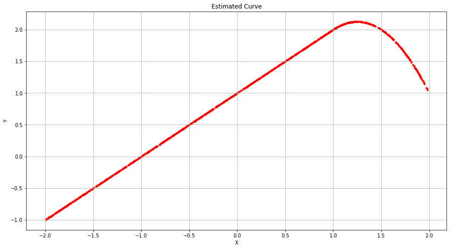
and obtain coefficient estimates $β_0 = 1, β_1 = 1, β_2 = −2$. Sketch the estimated curve between X = −2 and X = 2. Note the intercepts, slopes, and other relevant information.
Sol: The estimated curve is of the form $1+X$ for $X<1$ and $1+X -2(X-1)^2$ for $X \geq 1$.
import numpy as np
import matplotlib.pyplot as plt

def model(x):
    if x < 1:
        return 1+x
    else:
        return 1+x-2*((x-1)**2)

X = np.random.uniform(low=-2.0, high=2.0, size=1000)
vfunc = np.vectorize(model)
Y = vfunc(X)

fig = plt.figure(figsize=(15, 8))
ax = fig.add_subplot(111)
plt.scatter(X, Y, marker=".", color='r')
ax.set_xlabel('X')
ax.set_ylabel('Y')
ax.set_title('Estimated Curve')
plt.grid(b=True)
plt.show()
Q4. Suppose we fit a curve with basis functions $b_1(X) = I(0 ≤ X ≤ 2) − (X −1)I(1 ≤ X ≤ 2)$ and $b2(X) = (X −3)I(3 ≤ X ≤ 4)+I(4 < X ≤ 5)$. We fit the linear regression model
$$Y = β_0 + β_1b_1(X) + β_2b_2(X) + \epsilon$$
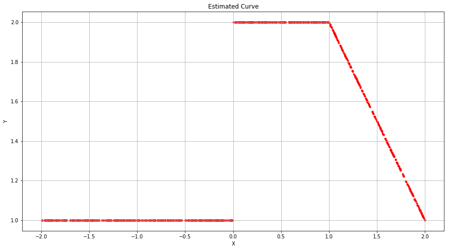
and obtain coefficient estimates $β_0 = 1, β_1 = 1, β_2 = 3$. Sketch the estimated curve between X = −2 and X = 2. Note the intercepts, slopes, and other relevant information.
def model(x):
    if x < 0:
        return 1.0
    elif x < 1:
        return 2.0
    else:
        return 3-x

X = np.random.uniform(low=-2.0, high=2.0, size=1000)
vfunc = np.vectorize(model)
Y = vfunc(X)

fig = plt.figure(figsize=(15, 8))
ax = fig.add_subplot(111)
plt.scatter(X, Y, marker=".", color='r')
ax.set_xlabel('X')
ax.set_ylabel('Y')
ax.set_title('Estimated Curve')
plt.grid(b=True)
plt.show()
Q5. Consider two curves, $\widehat{g_1}$ and $\widehat{g_2}$, defined by
$$\widehat{g} = argmin_g \bigg( \sum _{i=1}^{n}(y_i - g(x_i))^2 + \lambda \int \bigg[g^{(3)}(x) \bigg]^2 dx \bigg)$$
$$\widehat{g} = argmin_g \bigg( \sum _{i=1}^{n}(y_i - g(x_i))^2 + \lambda \int \bigg[g^{(4)}(x) \bigg]^2 dx \bigg)$$
where $g^{(m)}$ represents the $m$th derivative of $g$.
(a) As λ → ∞, will $\widehat{g_1}$ or $\widehat{g_2}$ have the smaller training RSS?
Sol: As $g_2$ is more flexible (as it has higher order penalty term), its training RSS will be smaller.
(b) As λ → ∞, will $\widehat{g_1}$ or $\widehat{g_2}$ have the smaller test RSS?
Sol: The test RSS will depend on the distribution of test data. If we have to provide the behaviour of test RSS based on the nature of curve, $\widehat{g_2}$ will have more test RSS as it is more flexible and hence may overfit the data.
(c) For λ = 0, will $\widehat{g_1}$ or $\widehat{g_2}$ have the smaller training and test RSS?
Sol: For $\lambda = 0$, $\widehat{g_1} = \widehat{g_2}$, as the smoothing effect is 0. Hence, both will have the same training and test RSS.