Tree-Based Methods
Tree-based methods stratify or segment the predictor space into a number of simple regions. To make a prediction, we use the mean or the mode of the training observations in the region in which the observation to be predicted belongs. The set of splitting rules can be summarized via a tree, these methods are also known as decision tree methods. Bagging, random forests and boosting produce multiple trees and then combine them in a single model to make the prediction. They provide improved accuracy at the cost of interpretability.
8.1 The Basics of Decision Trees
8.1.1 Regression Trees
Predicting Baseball Players’ Salaries Using Regression Trees
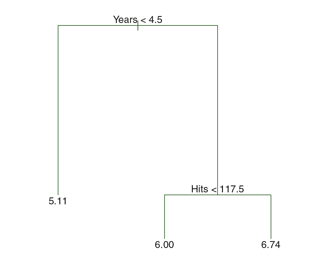
The regression tree which predicts the salary of baseball players is shown below. Regression tree consists of a series of splitting rules and stratifies or segments the players into three regions :
$$R_1 = {X \ | Years < 4.5}$$
$$R_2 = {X \ | Years \geq 4.5, Hits < 117.5}$$
$$R_3 = {X \ | Years \geq 4.5, Hits \geq 117.5}$$
The regions $R_1, R_2, R_3$ are known as terminal nodes or leaves. The points along the tree where the predictor space is split is called as internal nodes. The segments of the tree which connect the nodes are called branches. Regression trees are easier to interpret.
Prediction via Stratification of the Feature Space
The regression tree can be build by:
-
Dividing the predictor space $X_1, X_2, …, X_p$ into $J$ distinct and non-overlapping regions $R_1, R_2, …, R_J$.
-
Every observation that falls into region $R_j$, the prediction is simply the mean of the training observations in the region.
Theoretically, the regions can have any shape. In practice, the regions are divided into high dimensional rectangles for simplicity and ease of interpretation. The goal is to find the regions $R_1, R_2, …, R_J$ that minimizes
$$\sum _{j=1}^{J}\sum _{i \in R_j} (y_i - \widehat{y _{R_j}})^2$$
where $\widehat{y_{R_j}}$ is the mean of the training observation in the $j$th box. Predictors are split into regions by top-down greedy approach which is known as recursive binary splitting.
In recursive binary splitting, we first select a predictor $X_j$ and a cutpoint $s$, such that splitting the predictor space into region ${X|X_j < s}$ and ${X|X_j \geq s}$ leads to the greatest possible reduction in RSS. We consider all possible predictors $X_1, X_2, …, X_p$, and all possible cutpoints $s$ for each of the predictors and then choose the predictor and cutpoint that leads to lowest possible RSS. To be more specific, for any $j$ and $s$, the pair of half-planes are defined as:
$$R_1(j, s) = {X|X_j < s}$$
$$R_2(j, s) = {X|X_j \geq s}$$
and hence, we need to find the value of $j$ and $s$ which minimizes
$$\sum _{i: x_i \in R_1(j, s)} (y_i - \widehat{y _{R_1}})^2 + \sum _{i: x_i \in R_2(j, s)} (y_i - \widehat{y _{R_2}})^2$$
This process continues until a stopping criteria is reached (such as no regions contain more than 5 observations).
Tree Pruning
The process described above may lead to more complex trees and hence can result in overfitting. A smaller tree with fewer splits may lead to low variance and better at the cost of a little bias. One possible approach is to decide a threshold for decrease in RSS and split the tree only if that threshold is met. But there may be a case when seemingly worthless split early on may be followed by a good split that leads to a greater reduction in RSS. Hence a better approach is needed which build a large tree first and then prune it later to get a subtree. One way to prune the tree is by estimating test error for every possible subtrees (by crossvalidation) and then select the one which has the minimum test error. But this can be a cumbersome task as there can be a huge number of subtrees.
Cost complexity pruning or weakest link pruning instead considers a sequence of subtrees indexed by a nonnegative tuning parameter $\alpha$. For each value of $\alpha$, there exists a subtree $T \subset T_0$ such that
$$\sum _{m=1}^{|T|}\sum _{x_i \in R_m} (y_i - \widehat{y _{R_m}})^2 + \alpha \ \big|T \big|$$
is as small as possible. Here |T| indicates the number of inernal nodes in the tree T. The tuning parameter $\alpha$ controls the trade-off between the subtree’s fit to the training data and complexity. When $\alpha = 0$, the the subtree T will be equal to the largest tree $T_0$. When $\alpha$ increases, the subtrees with larger number of internal nodes will be penalized giving a smaller subtree as the fit. If we increase $\alpha$ from 0, branches get pruned out from the tree in a nested and predictable fashion and hence this entire process is quite efficient. The algorithm is as follows:
- Step 1: Use recursive binary splitting to obtain $T_0$.
- Step 2: Use cost complexity pruning to obtain a sequence of best subtrees as a function of $\alpha$.
- Step 2: Use K-fold crossvalidation and repeat Step 1 and 2 for all but the $k$th fold of the training data and obtain the validation MSE for the left-out $k$th fold for $k=1,2,3,…,K$. Finally pick $\alpha$ for whihc validation MSE is minimized.
- Step 4: Return the subtree from Step 2 which corresponds to the chosen value of $\alpha$.
8.1.2 Classification Trees
A classification tree is similar to a regression tree but instead of giving the mean of the regions as its prediction, it gives the most commonly occuring class of the training observations in the region as its prediction. For the interpretation purpose, in addition to the prediction, we may be interested in the class proportions for training observations in the regions as well.
Recursive binary spliiting can be used to build a classification tree as well. In a classification setting, we can not use RSS as a criterion for making the binary splits. Instead, we use classification error rate. Classification error for a region can be described as the fraction of the training observation that does not belong to the most common class for the region (mis-classified training observations). This can be given as:
$$E = 1 - max_k( \widehat{p} _{mk})$$
where $\widehat{p} _{mk}$ represents the proportion of the training observation in the $m$th region that belongs to the $k$th class. Classification error rate is not sufficiently sensitive for tree growing. Gini index is defined as:
$$G = \sum _{k=1}^{K} \widehat{p} _{mk}(1 - \widehat{p} _{mk})$$
is a measure of total variance across the $K$ classes. It can be observed that the Gini index takes a smaller value if all the $\widehat{p} _{mk}$ have values closer to 0 or 1. Hence, it can be viewed as a measure of node purity, as a small value of Gini index indicates that a node contains predominantly observations from a single class. Another measure is cross-entropy, which is given as:
$$D = - \sum _{k=1}^{K} \widehat{p} _{mk} log(\widehat{p} _{mk})$$
Cross-entroy has a similar behaviour as Gini index and they are quite similar numerically as well.
While building a tree, Gini index or Cross-entropy is used as the measure, as these measures are more sensitive to the node purity as compared to classification error rate. While pruning, classification error rate is preferred if prediction accuracy is the final goal.
There may be a case that in the classification tree, some splits seem redundant. For example, a split may lead to two leaves which has the exact same prediction (left leaf: 7 out of 11 in class A, right leaft: 9 out of 9 in class A). This split is done to achieve higher node purity. It has the advantage that if we encounter an observation that belongs to the right leaf(9 out of 9 in class A), we can be quite certain that the observation will belong to class A. But for the case of the observation belonging to the left leaf, we are less certain.
8.1.3 Trees Versus Linear Models
Simple linear models and regression tree models are quite different. Linear regression assumes a model of the form,
$$f(X) = \beta_0 + \sum _{j-1}^{p} X_j \beta_j$$
while regression trees have the form of
$$f(X) = \sum _{m=1}^{M}c_m \cdot 1 _{(X \in R_m)}$$
If relationship between the response and the predictors is linear, the linear model will work better. If there is a more comlex relationship, decision trees may outperform classical approaches.
8.1.4 Advantages and Disadvantages of Trees
Some of the advantages of decision tree approach is:
- easy interpretability.
- decision tree closely imitates the human decision-making process.
- can be decribed graphically and can be easily interpreted by non-experts.
- can easily handle qualitative variables (without making dummy variables).
Sometimes, decision tree aprooach may lead to lesser prediction accuracy though.