Applied
Solution 8:
(a) Perform linear regression on auto data with mpg as response and horsepower as the predictor and display the summary results.
import statsmodels.api as sm

X = sm.add_constant(auto[['horsepower']], prepend=True)
model = sm.OLS(auto['mpg'], X)
result = model.fit()
print(result.summary())
print("Prediction for horsepower 98: " +str(result.predict([1, 98])))
print("95% CI: " +str(result.conf_int(alpha=0.05, cols=None)))
                            OLS Regression Results
==============================================================================
Dep. Variable:                    mpg   R-squared:                       0.606
Model:                            OLS   Adj. R-squared:                  0.605
Method:                 Least Squares   F-statistic:                     599.7
Date:                Thu, 06 Sep 2018   Prob (F-statistic):           7.03e-81
Time:                        21:37:43   Log-Likelihood:                -1178.7
No. Observations:                 392   AIC:                             2361.
Df Residuals:                     390   BIC:                             2369.
Df Model:                           1
Covariance Type:            nonrobust
==============================================================================
                 coef    std err          t      P>|t|      [0.025      0.975]
------------------------------------------------------------------------------
const         39.9359      0.717     55.660      0.000      38.525      41.347
horsepower    -0.1578      0.006    -24.489      0.000      -0.171      -0.145
==============================================================================
Omnibus:                       16.432   Durbin-Watson:                   0.920
Prob(Omnibus):                  0.000   Jarque-Bera (JB):               17.305
Skew:                           0.492   Prob(JB):                     0.000175
Kurtosis:                       3.299   Cond. No.                         322.
==============================================================================

Warnings:
[1] Standard Errors assume that the covariance matrix of the errors is correctly specified.
Prediction for horsepower 98: [24.46707715]
95% CI:                     0          1
const       38.525212  41.346510
horsepower  -0.170517  -0.145172
i. Is there a relationship between the predictor and the response?
Yes
ii. How strong is the relationship between the predictor and the response?
As the value of $R^2$-statistic is 0.606, which means that 60% variability is explained by the model.
iii. Is the relationship between the predictor and the response positive or negative?
Negative coefficient denotes negative relationship.
iv. What is the predicted mpg associated with a horsepower of 98? What are the associated 95% confidence and prediction intervals?
The value of mpg for horsepower = 98 is 24.4671.
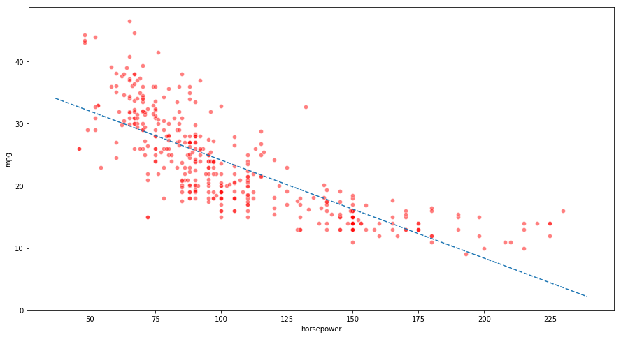
(b) Plot the response and the predictor. Also show the regression line.
import matplotlib.pyplot as plt
import numpy as np

fig = plt.figure(figsize=(15,8))
ax = fig.add_subplot(111)

ax = sns.scatterplot(x="horsepower", y="mpg", color='r', alpha=0.5, data=auto)

x_vals = np.array(ax.get_xlim())
y_vals = 39.9359 - 0.1578 * x_vals
plt.plot(x_vals, y_vals, '--')
[<matplotlib.lines.Line2D at 0x11a222048>]
Solution 9:
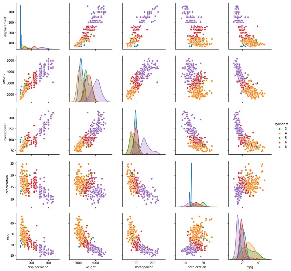
(a) Produce a scatterplot matrix which includes all of the variables in the data set.
# Scatter plot of quantitative variables
sns.pairplot(auto, vars=['displacement', 'weight', 'horsepower', 'acceleration', 'mpg'], hue='cylinders')
/Users/amitrajan/Desktop/PythonVirtualEnv/Python3_VirtualEnv/lib/python3.6/site-packages/scipy/stats/stats.py:1713: FutureWarning: Using a non-tuple sequence for multidimensional indexing is deprecated; use `arr[tuple(seq)]` instead of `arr[seq]`. In the future this will be interpreted as an array index, `arr[np.array(seq)]`, which will result either in an error or a different result.
  return np.add.reduce(sorted[indexer] * weights, axis=axis) / sumval


<seaborn.axisgrid.PairGrid at 0x11a1c4f98>
(b) Compute the matrix of correlations between the variables.
auto.corr()
| mpg | cylinders | displacement | horsepower | weight | acceleration | year | origin | |
|---|---|---|---|---|---|---|---|---|
| mpg | 1.000000 | -0.777618 | -0.805127 | -0.778427 | -0.832244 | 0.423329 | 0.580541 | 0.565209 |
| cylinders | -0.777618 | 1.000000 | 0.950823 | 0.842983 | 0.897527 | -0.504683 | -0.345647 | -0.568932 |
| displacement | -0.805127 | 0.950823 | 1.000000 | 0.897257 | 0.932994 | -0.543800 | -0.369855 | -0.614535 |
| horsepower | -0.778427 | 0.842983 | 0.897257 | 1.000000 | 0.864538 | -0.689196 | -0.416361 | -0.455171 |
| weight | -0.832244 | 0.897527 | 0.932994 | 0.864538 | 1.000000 | -0.416839 | -0.309120 | -0.585005 |
| acceleration | 0.423329 | -0.504683 | -0.543800 | -0.689196 | -0.416839 | 1.000000 | 0.290316 | 0.212746 |
| year | 0.580541 | -0.345647 | -0.369855 | -0.416361 | -0.309120 | 0.290316 | 1.000000 | 0.181528 |
| origin | 0.565209 | -0.568932 | -0.614535 | -0.455171 | -0.585005 | 0.212746 | 0.181528 | 1.000000 |
(c) Perform a multiple linear regression with mpg as the response and all other variables except name as the predictors.
X = auto[['cylinders', 'displacement', 'horsepower', 'weight', 'acceleration', 'year', 'origin']]
X = sm.add_constant(X, prepend=True)
y = auto['mpg']

model = sm.OLS(y, X)
result = model.fit()
print(result.summary())
                            OLS Regression Results
==============================================================================
Dep. Variable:                    mpg   R-squared:                       0.821
Model:                            OLS   Adj. R-squared:                  0.818
Method:                 Least Squares   F-statistic:                     252.4
Date:                Mon, 10 Sep 2018   Prob (F-statistic):          2.04e-139
Time:                        19:11:35   Log-Likelihood:                -1023.5
No. Observations:                 392   AIC:                             2063.
Df Residuals:                     384   BIC:                             2095.
Df Model:                           7
Covariance Type:            nonrobust
================================================================================
                   coef    std err          t      P>|t|      [0.025      0.975]
--------------------------------------------------------------------------------
const          -17.2184      4.644     -3.707      0.000     -26.350      -8.087
cylinders       -0.4934      0.323     -1.526      0.128      -1.129       0.142
displacement     0.0199      0.008      2.647      0.008       0.005       0.035
horsepower      -0.0170      0.014     -1.230      0.220      -0.044       0.010
weight          -0.0065      0.001     -9.929      0.000      -0.008      -0.005
acceleration     0.0806      0.099      0.815      0.415      -0.114       0.275
year             0.7508      0.051     14.729      0.000       0.651       0.851
origin           1.4261      0.278      5.127      0.000       0.879       1.973
==============================================================================
Omnibus:                       31.906   Durbin-Watson:                   1.309
Prob(Omnibus):                  0.000   Jarque-Bera (JB):               53.100
Skew:                           0.529   Prob(JB):                     2.95e-12
Kurtosis:                       4.460   Cond. No.                     8.59e+04
==============================================================================

Warnings:
[1] Standard Errors assume that the covariance matrix of the errors is correctly specified.
[2] The condition number is large, 8.59e+04. This might indicate that there are
strong multicollinearity or other numerical problems.
i. Is there a relationship between the predictors and the response?
As the $R^2$-statistic is 0.821, we can say that 82% variability is explained by the model.
ii. Which predictors appear to have a statistically significant relationship to the response?
The predictors that have statistically significant relationship to the response are: displacement, weight, year and origin.
iii. What does the coefficient for the year variable suggest?
The coefficient of year varaible suggests that if all the other predictors are kept constant, increase of 1 in year results in 0.7508 increase in mpg.
(e) Fit linear regression models with interaction effects. Do any interactions appear to be statistically significant?
auto['cylinders_displacement'] = auto['cylinders']*auto['displacement']
auto['horsepower_displacement'] = auto['horsepower']*auto['displacement']
auto['weight_displacement'] = auto['weight']*auto['displacement']

X = auto[['cylinders', 'displacement', 'horsepower', 'weight', 'acceleration', 'year', 'origin',
          'cylinders_displacement', 'horsepower_displacement', 'weight_displacement']]
X = sm.add_constant(X, prepend=True)
y = auto['mpg']

model = sm.OLS(y, X)
result = model.fit()
print(result.summary())
                            OLS Regression Results
==============================================================================
Dep. Variable:                    mpg   R-squared:                       0.866
Model:                            OLS   Adj. R-squared:                  0.862
Method:                 Least Squares   F-statistic:                     246.0
Date:                Thu, 06 Sep 2018   Prob (F-statistic):          1.96e-159
Time:                        21:37:48   Log-Likelihood:                -967.41
No. Observations:                 392   AIC:                             1957.
Df Residuals:                     381   BIC:                             2000.
Df Model:                          10
Covariance Type:            nonrobust
===========================================================================================
                              coef    std err          t      P>|t|      [0.025      0.975]
-------------------------------------------------------------------------------------------
const                      -2.4166      4.438     -0.545      0.586     -11.142       6.309
cylinders                   0.8214      0.618      1.329      0.185      -0.394       2.037
displacement               -0.0778      0.013     -5.822      0.000      -0.104      -0.052
horsepower                 -0.1488      0.029     -5.222      0.000      -0.205      -0.093
weight                     -0.0062      0.001     -4.443      0.000      -0.009      -0.003
acceleration               -0.1312      0.097     -1.357      0.175      -0.321       0.059
year                        0.7566      0.045     16.822      0.000       0.668       0.845
origin                      0.5797      0.258      2.247      0.025       0.072       1.087
cylinders_displacement     -0.0014      0.003     -0.516      0.606      -0.007       0.004
horsepower_displacement     0.0004   8.27e-05      4.481      0.000       0.000       0.001
weight_displacement      1.046e-05   4.37e-06      2.393      0.017    1.87e-06     1.9e-05
==============================================================================
Omnibus:                       47.260   Durbin-Watson:                   1.507
Prob(Omnibus):                  0.000   Jarque-Bera (JB):               97.455
Skew:                           0.662   Prob(JB):                     6.89e-22
Kurtosis:                       5.053   Cond. No.                     2.56e+07
==============================================================================

Warnings:
[1] Standard Errors assume that the covariance matrix of the errors is correctly specified.
[2] The condition number is large, 2.56e+07. This might indicate that there are
strong multicollinearity or other numerical problems.
Interactions of horsepower and displacement and weight and displacement have significant effect.
Solution 10: This question should be answered using the Carseats data set.
(a) Fit a multiple regression model to predict Sales using Price, Urban, and US.
carsets = pd.read_csv("data/Carsets.csv")
carsets['US'] = carsets['US'].map({'Yes': 1, 'No': 0})
carsets['Urban'] = carsets['Urban'].map({'Yes': 1, 'No': 0})

X = carsets[['Price', 'Urban', 'US']]
X = sm.add_constant(X, prepend=True)
y = carsets['Sales']

model = sm.OLS(y, X)
result = model.fit()
print(result.summary())
                            OLS Regression Results
==============================================================================
Dep. Variable:                  Sales   R-squared:                       0.239
Model:                            OLS   Adj. R-squared:                  0.234
Method:                 Least Squares   F-statistic:                     41.52
Date:                Thu, 06 Sep 2018   Prob (F-statistic):           2.39e-23
Time:                        21:37:48   Log-Likelihood:                -927.66
No. Observations:                 400   AIC:                             1863.
Df Residuals:                     396   BIC:                             1879.
Df Model:                           3
Covariance Type:            nonrobust
==============================================================================
                 coef    std err          t      P>|t|      [0.025      0.975]
------------------------------------------------------------------------------
const         13.0435      0.651     20.036      0.000      11.764      14.323
Price         -0.0545      0.005    -10.389      0.000      -0.065      -0.044
Urban         -0.0219      0.272     -0.081      0.936      -0.556       0.512
US             1.2006      0.259      4.635      0.000       0.691       1.710
==============================================================================
Omnibus:                        0.676   Durbin-Watson:                   1.912
Prob(Omnibus):                  0.713   Jarque-Bera (JB):                0.758
Skew:                           0.093   Prob(JB):                        0.684
Kurtosis:                       2.897   Cond. No.                         628.
==============================================================================

Warnings:
[1] Standard Errors assume that the covariance matrix of the errors is correctly specified.
(b) Provide an interpretation of each coefficient in the model. Be careful—some of the variables in the model are qualitative!
Sales decreases by 0.0545 per unit increase in Price given that all the other predictors are not changed. Urban has no significant effect on the response. If all the other predictors are constant, being a US car increases the Sales by average of 1.2006.
(c) Write out the model in equation form, being careful to handle the qualitative variables properly.
The model in equation form is as follows:
$$Sales = 13.0435 - 0.0545 \times Price + 1.2006 - 0.0219 \ (if \ US, Urban)$$ $$Sales = 13.0435 - 0.0545 \times Price + 1.2006 \ (if \ US, \ not \ Urban)$$ $$Sales = 13.0435 - 0.0545 \times Price - 0.0219 \ (if \ not \ US, Urban)$$ $$Sales = 13.0435 - 0.0545 \times Price \ (if \ not \ US, not \ Urban)$$
(d) For which of the predictors can you reject the null hypothesis H0 : βj = 0?
We can reject the null hypothesis for Price and US.
(e) On the basis of your response to the previous question, fit a smaller model that only uses the predictors for which there is evidence of association with the outcome.
X = carsets[['Price', 'US']]
X = sm.add_constant(X, prepend=True)
y = carsets['Sales']

model = sm.OLS(y, X)
result = model.fit()
print(result.summary())
                            OLS Regression Results
==============================================================================
Dep. Variable:                  Sales   R-squared:                       0.239
Model:                            OLS   Adj. R-squared:                  0.235
Method:                 Least Squares   F-statistic:                     62.43
Date:                Thu, 06 Sep 2018   Prob (F-statistic):           2.66e-24
Time:                        21:37:48   Log-Likelihood:                -927.66
No. Observations:                 400   AIC:                             1861.
Df Residuals:                     397   BIC:                             1873.
Df Model:                           2
Covariance Type:            nonrobust
==============================================================================
                 coef    std err          t      P>|t|      [0.025      0.975]
------------------------------------------------------------------------------
const         13.0308      0.631     20.652      0.000      11.790      14.271
Price         -0.0545      0.005    -10.416      0.000      -0.065      -0.044
US             1.1996      0.258      4.641      0.000       0.692       1.708
==============================================================================
Omnibus:                        0.666   Durbin-Watson:                   1.912
Prob(Omnibus):                  0.717   Jarque-Bera (JB):                0.749
Skew:                           0.092   Prob(JB):                        0.688
Kurtosis:                       2.895   Cond. No.                         607.
==============================================================================

Warnings:
[1] Standard Errors assume that the covariance matrix of the errors is correctly specified.
(f) How well do the models in (a) and (e) fit the data?
If we see the $R^2$-statistic of the models, for both the models, it has a value of 0.239. Hence both the models explains 23.9% variability in data and model in (a), which has one more predictor does not improve over accuracy.
(g) Using the model from (e), obtain 95% confidence intervals for the coefficient(s).
The 95% confidence intervals for the coefficients are:
- Intercept : [11.7688, 14.2928]
- Price : [-0.0555, 0.0535]
- US : [0.6836, 1.7156]
Solution 11. In this problem we will investigate the t-statistic for the null hypothesis H0 : β = 0 in simple linear regression without an intercept. To begin, we generate a predictor x and a response y as:
import random

random.seed(1)
x = np.random.normal(loc=0, scale=1, size=100)
y = 2*x + np.random.normal(loc=0, scale=1, size=100)
(a) Perform a simple linear regression of y onto x, without an intercept. Report the coefficient estimate $\widehat{\beta}$, the standard error of this coefficient estimate, and the t-statistic and p-value associated with the null hypothesis H0 : β = 0. Comment on these results.
model = sm.OLS(y, x)
result = model.fit()
print(result.summary())
                            OLS Regression Results
==============================================================================
Dep. Variable:                      y   R-squared:                       0.765
Model:                            OLS   Adj. R-squared:                  0.763
Method:                 Least Squares   F-statistic:                     322.1
Date:                Thu, 06 Sep 2018   Prob (F-statistic):           6.90e-33
Time:                        21:37:48   Log-Likelihood:                -136.69
No. Observations:                 100   AIC:                             275.4
Df Residuals:                      99   BIC:                             278.0
Df Model:                           1
Covariance Type:            nonrobust
==============================================================================
                 coef    std err          t      P>|t|      [0.025      0.975]
------------------------------------------------------------------------------
x1             1.8076      0.101     17.946      0.000       1.608       2.007
==============================================================================
Omnibus:                        0.587   Durbin-Watson:                   1.969
Prob(Omnibus):                  0.746   Jarque-Bera (JB):                0.714
Skew:                          -0.083   Prob(JB):                        0.700
Kurtosis:                       2.620   Cond. No.                         1.00
==============================================================================

Warnings:
[1] Standard Errors assume that the covariance matrix of the errors is correctly specified.
Coefficient estimate is 1.9766 with a standard error of 0.099. The t-statistic associated with null hypothesis is 19.900 which gives a significantly low p-value. The $R^2$-statistic, whose value is 0.800, suggests that the predictor is significant and explains 80% of the variability.
(b) Now perform a simple linear regression of x onto y without an intercept, and report the coefficient estimate, its standard error, and the corresponding t-statistic and p-values associated with the null hypothesis H0 : β = 0. Comment on these results.
model = sm.OLS(x, y)
result = model.fit()
print(result.summary())
                            OLS Regression Results
==============================================================================
Dep. Variable:                      y   R-squared:                       0.765
Model:                            OLS   Adj. R-squared:                  0.763
Method:                 Least Squares   F-statistic:                     322.1
Date:                Thu, 06 Sep 2018   Prob (F-statistic):           6.90e-33
Time:                        21:37:48   Log-Likelihood:                -64.089
No. Observations:                 100   AIC:                             130.2
Df Residuals:                      99   BIC:                             132.8
Df Model:                           1
Covariance Type:            nonrobust
==============================================================================
                 coef    std err          t      P>|t|      [0.025      0.975]
------------------------------------------------------------------------------
x1             0.4232      0.024     17.946      0.000       0.376       0.470
==============================================================================
Omnibus:                        0.724   Durbin-Watson:                   1.990
Prob(Omnibus):                  0.696   Jarque-Bera (JB):                0.841
Skew:                           0.179   Prob(JB):                        0.657
Kurtosis:                       2.729   Cond. No.                         1.00
==============================================================================

Warnings:
[1] Standard Errors assume that the covariance matrix of the errors is correctly specified.
Coefficient estimate is 0.4048 with a standard error of 0.020. The t-statistic associated with null hypothesis is 19.900 which gives a significantly low p-value. The $R^2$-statistic, whose value is 0.800, suggests that the predictor is significant and explains 80% of the variability.
(c) What is the relationship between the results obtained in (a) and (b)?
The coefficients for the two models follow inverse relationship. The t-statistic and $R^2$-statistic are same.
Solution 12: This problem involves simple linear regression without an intercept.
(a) Recall that the coefficient estimate $\widehat{\beta}$ for the linear regression of Y onto X without an intercept is given by:
$$\widehat{\beta} = \frac{\sum _{i=1}^{n}x_i y_i}{\sum _{i^{’}=1}^{n}x _{i^{’}}^2}$$
Under what circumstance is the coefficient estimate for the regression of X onto Y the same as the coefficient estimate for the regression of Y onto X?
The coefficients will be same when:
$$\sum _{i=1}^{n}x _{i}^2 = \sum _{i=1}^{n}y _{i}^2$$
(c) Generate an example with n = 100 observations in which the coefficient estimate for the regression of X onto Y is the same as the coefficient estimate for the regression of Y onto X.
random.seed(1)
x = np.random.normal(loc=0, scale=1, size=100)
y = np.random.normal(loc=0, scale=1, size=100)
print(np.sum(x**2))
print(np.sum(y**2))

model = sm.OLS(y, x)
result = model.fit()
print(result.summary())

print("\n \n")

model = sm.OLS(x, y)
result = model.fit()
print(result.summary())
83.09270311310463
121.64942659232169
                            OLS Regression Results
==============================================================================
Dep. Variable:                      y   R-squared:                       0.000
Model:                            OLS   Adj. R-squared:                 -0.010
Method:                 Least Squares   F-statistic:                  0.004235
Date:                Thu, 06 Sep 2018   Prob (F-statistic):              0.948
Time:                        21:37:48   Log-Likelihood:                -151.69
No. Observations:                 100   AIC:                             305.4
Df Residuals:                      99   BIC:                             308.0
Df Model:                           1
Covariance Type:            nonrobust
==============================================================================
                 coef    std err          t      P>|t|      [0.025      0.975]
------------------------------------------------------------------------------
x1            -0.0079      0.122     -0.065      0.948      -0.249       0.233
==============================================================================
Omnibus:                        2.389   Durbin-Watson:                   1.875
Prob(Omnibus):                  0.303   Jarque-Bera (JB):                1.867
Skew:                          -0.319   Prob(JB):                        0.393
Kurtosis:                       3.205   Cond. No.                         1.00
==============================================================================

Warnings:
[1] Standard Errors assume that the covariance matrix of the errors is correctly specified.


                            OLS Regression Results
==============================================================================
Dep. Variable:                      y   R-squared:                       0.000
Model:                            OLS   Adj. R-squared:                 -0.010
Method:                 Least Squares   F-statistic:                  0.004235
Date:                Thu, 06 Sep 2018   Prob (F-statistic):              0.948
Time:                        21:37:48   Log-Likelihood:                -132.63
No. Observations:                 100   AIC:                             267.3
Df Residuals:                      99   BIC:                             269.9
Df Model:                           1
Covariance Type:            nonrobust
==============================================================================
                 coef    std err          t      P>|t|      [0.025      0.975]
------------------------------------------------------------------------------
x1            -0.0054      0.083     -0.065      0.948      -0.170       0.159
==============================================================================
Omnibus:                        5.314   Durbin-Watson:                   1.818
Prob(Omnibus):                  0.070   Jarque-Bera (JB):                5.119
Skew:                           0.554   Prob(JB):                       0.0773
Kurtosis:                       3.012   Cond. No.                         1.00
==============================================================================

Warnings:
[1] Standard Errors assume that the covariance matrix of the errors is correctly specified.
Solution 13: In this exercise you will create some simulated data and will fit simple linear regression models to it. Make sure to use set.seed(1) prior to starting part (a) to ensure consistent results.
random.seed(1)
(a) Create a vector, x, containing 100 observations drawn from a N(0, 1) distribution. This represents a feature, X.
X = np.random.normal(loc=0, scale=1, size=100)
(b) Create a vector, eps, containing 100 observations drawn from a N(0, 0.25) distribution i.e. a normal distribution with mean zero and variance 0.25.
eps = np.random.normal(loc=0, scale=0.25, size=100)
(c) Using X and eps, generate a vector y according to the model $Y = −1 + 0.5X + \epsilon$. What is the length of the vector Y? What are the values of β0 and β1 in this linear model?
Y = -1 + (0.5*X) + eps
print("Length of Y:" +str(len(Y)))
Length of Y:100
Lengt of Y is 100. The values of $\beta_0$ and $\beta_1$ are -1 and 0.5 respectively.
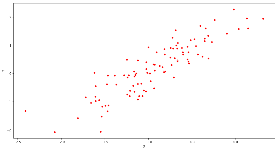
(d) Create a scatterplot displaying the relationship between x and y. Comment on what you observe.
fig = plt.figure(figsize=(15,8))
ax = fig.add_subplot(111)
ax = sns.scatterplot(Y, X, color='r')

ax.set_xlabel("X")
ax.set_ylabel("Y")
plt.show()
(e) Fit a least squares linear model to predict y using x. Comment on the model obtained. How do $\widehat{\beta_0}$ and $\widehat{\beta_1}$ compare to β0 and β1?
The values of $\widehat\beta_0$ and $\widehat\beta_1$ are -1.0145 and 0.5130 respectively. They are quite similar to $\beta_0$ and $\beta_1$.
X_1 = sm.add_constant(X, prepend=True)
model = sm.OLS(Y, X_1)
result = model.fit()
print(result.summary())
                            OLS Regression Results
==============================================================================
Dep. Variable:                      y   R-squared:                       0.772
Model:                            OLS   Adj. R-squared:                  0.770
Method:                 Least Squares   F-statistic:                     332.6
Date:                Thu, 06 Sep 2018   Prob (F-statistic):           2.89e-33
Time:                        21:37:49   Log-Likelihood:                 3.2646
No. Observations:                 100   AIC:                            -2.529
Df Residuals:                      98   BIC:                             2.681
Df Model:                           1
Covariance Type:            nonrobust
==============================================================================
                 coef    std err          t      P>|t|      [0.025      0.975]
------------------------------------------------------------------------------
const         -1.0103      0.024    -41.824      0.000      -1.058      -0.962
x1             0.4691      0.026     18.237      0.000       0.418       0.520
==============================================================================
Omnibus:                        4.700   Durbin-Watson:                   2.124
Prob(Omnibus):                  0.095   Jarque-Bera (JB):                4.057
Skew:                          -0.464   Prob(JB):                        0.132
Kurtosis:                       3.336   Cond. No.                         1.24
==============================================================================

Warnings:
[1] Standard Errors assume that the covariance matrix of the errors is correctly specified.
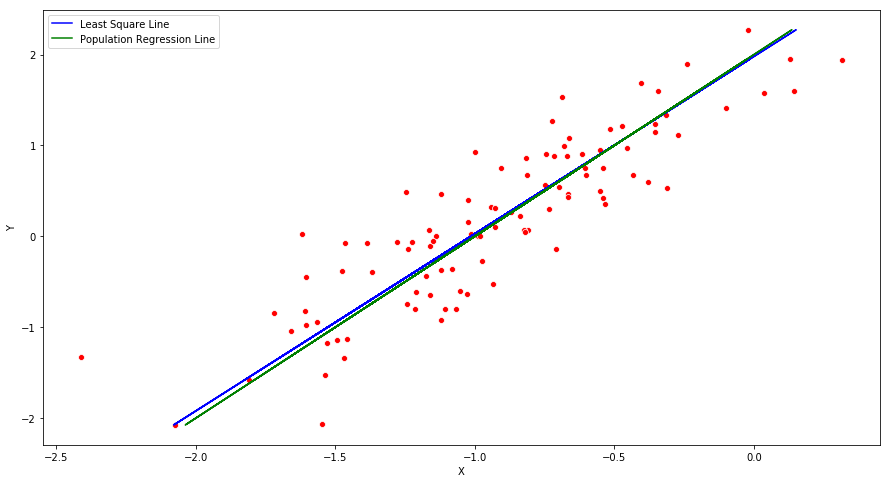
(f) Display the least squares line on the scatterplot obtained in (d). Draw the population regression line on the plot, in a different color. Use the legend() command to create an appropriate legend.
fig = plt.figure(figsize=(15,8))
ax = fig.add_subplot(111)
ax = sns.scatterplot(Y, X, color='r')

y_hat = -1.0145 + (0.5130 * X)
plt.plot(y_hat, X, color='blue', label="Least Square Line")

y_population = -1 + (0.5 * X)
plt.plot(y_population, X, color='green', label="Population Regression Line")

ax.set_xlabel("X")
ax.set_ylabel("Y")
ax.legend()

plt.show()
(g) Now fit a polynomial regression model that predicts y using x and $x^2$. Is there evidence that the quadratic term improves the model fit? Explain your answer.
As the p-value for the predictor $x^2$ is 0.644, it is not significant. The $R^2$-statistic has not improved much as well.
X_2 = X**2
X_pol = np.stack((X, X_2), axis=-1)

X_pol = sm.add_constant(X_pol, prepend=True)
model = sm.OLS(Y, X_pol)
result = model.fit()
print(result.summary())
                            OLS Regression Results
==============================================================================
Dep. Variable:                      y   R-squared:                       0.775
Model:                            OLS   Adj. R-squared:                  0.770
Method:                 Least Squares   F-statistic:                     167.1
Date:                Thu, 06 Sep 2018   Prob (F-statistic):           3.73e-32
Time:                        21:37:49   Log-Likelihood:                 3.8606
No. Observations:                 100   AIC:                            -1.721
Df Residuals:                      97   BIC:                             6.094
Df Model:                           2
Covariance Type:            nonrobust
==============================================================================
                 coef    std err          t      P>|t|      [0.025      0.975]
------------------------------------------------------------------------------
const         -1.0301      0.030    -33.950      0.000      -1.090      -0.970
x1             0.4630      0.026     17.592      0.000       0.411       0.515
x2             0.0238      0.022      1.078      0.283      -0.020       0.068
==============================================================================
Omnibus:                        5.916   Durbin-Watson:                   2.203
Prob(Omnibus):                  0.052   Jarque-Bera (JB):                5.290
Skew:                          -0.522   Prob(JB):                       0.0710
Kurtosis:                       3.424   Cond. No.                         2.33
==============================================================================

Warnings:
[1] Standard Errors assume that the covariance matrix of the errors is correctly specified.
Solution 14: This problem focuses on the collinearity problem.
(a) Generate data by following R command:
- set .seed (1)
- x1=runif (100)
- x2 =0.5* x1+rnorm (100) /10
- y=2+2* x1 +0.3* x2+rnorm (100)
The last line corresponds to creating a linear model in which y is a function of x1 and x2. Write out the form of the linear model. What are the regression coefficients?
The linear model is:
$$ Y = 2 + 2 \times X1 + 0.3 \times X2 + \epsilon$$
The regression coefficients are 2,2 and 0.3.
random.seed(1)
X1 = np.random.normal(loc=0, scale=1, size=100)
X2 = 0.5*X1 + (np.random.normal(loc=0, scale=1, size=100)/10)
Y = 2 + (2*X1) + (0.3*X2) + (np.random.normal(loc=0, scale=1, size=100))
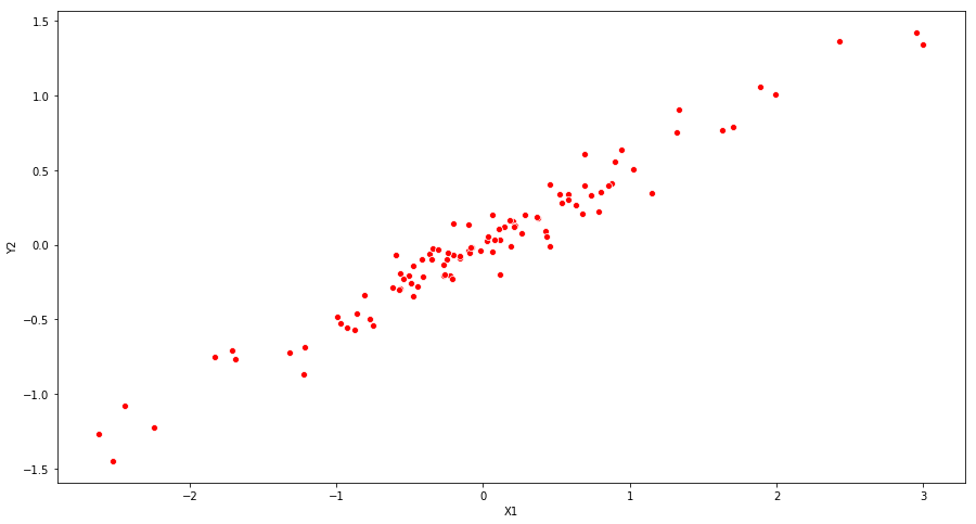
(b) What is the correlation between X1 and X2? Create a scatterplot displaying the relationship between the variables.
The correlation coefficient between X1 and X2 is 0.9836387796085876. The scatterplot shows the same tendency.
print("Correlation coefficient: " + str(np.corrcoef(X1, X2)[0][1]))
fig = plt.figure(figsize=(15,8))
ax = fig.add_subplot(111)
ax = sns.scatterplot(x=X1, y=X2, color='r')

ax.set_xlabel("X1")
ax.set_ylabel("Y2")

plt.show()
Correlation coefficient: 0.9773524295882932
(c) Using this data, fit a least squares regression to predict y using x1 and x2. Describe the results obtained. What are $\widehat{\beta_0}, \widehat{\beta_1}, \widehat{\beta_2}$? How do these relate to the true β0, β1, and β2? Can you reject the null hypothesis H0 : β1 = 0? How about the null hypothesis H0 : β2 = 0?
The values of $\widehat{\beta_0}, \widehat{\beta_1}, \widehat{\beta_2}$ are 1.8824, 1.1253 and 2.0781. We can reject the null hypothesis for $\widehat{\beta_0}$ and $\widehat{\beta_1}$ as p-values are less than 0.05. If we increase the level of confidence to 0.01, the null hypothesis for $\widehat{\beta_1}$ can not be rejected.
X = np.stack((X1, X2), axis=-1)
X = sm.add_constant(X, prepend=True)

model = sm.OLS(Y, X)
result = model.fit()
print(result.summary())
                            OLS Regression Results
==============================================================================
Dep. Variable:                      y   R-squared:                       0.841
Model:                            OLS   Adj. R-squared:                  0.837
Method:                 Least Squares   F-statistic:                     255.6
Date:                Thu, 06 Sep 2018   Prob (F-statistic):           2.15e-39
Time:                        21:37:49   Log-Likelihood:                -137.49
No. Observations:                 100   AIC:                             281.0
Df Residuals:                      97   BIC:                             288.8
Df Model:                           2
Covariance Type:            nonrobust
==============================================================================
                 coef    std err          t      P>|t|      [0.025      0.975]
------------------------------------------------------------------------------
const          2.0716      0.097     21.300      0.000       1.879       2.265
x1             1.8083      0.457      3.956      0.000       0.901       2.716
x2             0.7538      0.893      0.845      0.400      -1.018       2.525
==============================================================================
Omnibus:                        0.011   Durbin-Watson:                   2.033
Prob(Omnibus):                  0.995   Jarque-Bera (JB):                0.108
Skew:                           0.021   Prob(JB):                        0.947
Kurtosis:                       2.844   Cond. No.                         11.6
==============================================================================

Warnings:
[1] Standard Errors assume that the covariance matrix of the errors is correctly specified.
(d) Now fit a least squares regression to predict y using only x1. Comment on your results. Can you reject the null hypothesis H0 : β1 = 0?
The values of $\widehat{\beta_0}$ and $\widehat{\beta_1}$ are 1.8988 and 2.1601. We can reject the null hypothesis for $\widehat{\beta_1}$ as p-value is very low.
X = sm.add_constant(X1, prepend=True)

model = sm.OLS(Y, X)
result = model.fit()
print(result.summary())
                            OLS Regression Results
==============================================================================
Dep. Variable:                      y   R-squared:                       0.839
Model:                            OLS   Adj. R-squared:                  0.838
Method:                 Least Squares   F-statistic:                     512.0
Date:                Thu, 06 Sep 2018   Prob (F-statistic):           1.07e-40
Time:                        21:37:49   Log-Likelihood:                -137.85
No. Observations:                 100   AIC:                             279.7
Df Residuals:                      98   BIC:                             284.9
Df Model:                           1
Covariance Type:            nonrobust
==============================================================================
                 coef    std err          t      P>|t|      [0.025      0.975]
------------------------------------------------------------------------------
const          2.0752      0.097     21.390      0.000       1.883       2.268
x1             2.1856      0.097     22.628      0.000       1.994       2.377
==============================================================================
Omnibus:                        0.020   Durbin-Watson:                   1.985
Prob(Omnibus):                  0.990   Jarque-Bera (JB):                0.152
Skew:                          -0.009   Prob(JB):                        0.927
Kurtosis:                       2.810   Cond. No.                         1.01
==============================================================================

Warnings:
[1] Standard Errors assume that the covariance matrix of the errors is correctly specified.
(e) Now fit a least squares regression to predict y using only x2. Comment on your results. Can you reject the null hypothesis H0 : β1 = 0?
The values of $\widehat{\beta_0}$ and $\widehat{\beta_1}$ are 1.8606 and 4.2647. We can reject the null hypothesis for $\widehat{\beta_1}$ as p-value is very low.
X = sm.add_constant(X2, prepend=True)

model = sm.OLS(Y, X)
result = model.fit()
print(result.summary())
                            OLS Regression Results
==============================================================================
Dep. Variable:                      y   R-squared:                       0.815
Model:                            OLS   Adj. R-squared:                  0.813
Method:                 Least Squares   F-statistic:                     431.1
Date:                Thu, 06 Sep 2018   Prob (F-statistic):           1.16e-37
Time:                        21:37:49   Log-Likelihood:                -144.97
No. Observations:                 100   AIC:                             293.9
Df Residuals:                      98   BIC:                             299.1
Df Model:                           1
Covariance Type:            nonrobust
==============================================================================
                 coef    std err          t      P>|t|      [0.025      0.975]
------------------------------------------------------------------------------
const          2.0543      0.104     19.721      0.000       1.848       2.261
x1             4.2050      0.203     20.764      0.000       3.803       4.607
==============================================================================
Omnibus:                        0.125   Durbin-Watson:                   2.209
Prob(Omnibus):                  0.939   Jarque-Bera (JB):                0.188
Skew:                           0.081   Prob(JB):                        0.910
Kurtosis:                       2.864   Cond. No.                         1.94
==============================================================================

Warnings:
[1] Standard Errors assume that the covariance matrix of the errors is correctly specified.
(f) Do the results obtained in (c)–(e) contradict each other? Explain your answer.
In case of collinearity, t-statistic declines and consequently we may fail to reject the null hypothesis. This is the case for $\widehat{\beta_2}$ in (c). For the model in (c), the standard errors corresponding to $\beta$s are high and hence the t-statistic does not capture the accurate behaviour.
Solution 15: This problem involves the Boston data set, which we saw in the lab for this chapter. We will now try to predict per capita crime rate using the other variables in this data set. In other words, per capita crime rate is the response, and the other variables are the predictors.
from sklearn.datasets import load_boston

boston = load_boston()
df_boston = pd.DataFrame(boston.data, columns=['CRIM', 'ZN', 'INDUS', 'CHAS', 'NOX', 'RM', 'AGE', 'DIS', 'RAD', 'TAX',
                                               'PTRATIO', 'B', 'LSTAT'])
df_boston.head()
| CRIM | ZN | INDUS | CHAS | NOX | RM | AGE | DIS | RAD | TAX | PTRATIO | B | LSTAT | |
|---|---|---|---|---|---|---|---|---|---|---|---|---|---|
| 0 | 0.00632 | 18.0 | 2.31 | 0.0 | 0.538 | 6.575 | 65.2 | 4.0900 | 1.0 | 296.0 | 15.3 | 396.90 | 4.98 |
| 1 | 0.02731 | 0.0 | 7.07 | 0.0 | 0.469 | 6.421 | 78.9 | 4.9671 | 2.0 | 242.0 | 17.8 | 396.90 | 9.14 |
| 2 | 0.02729 | 0.0 | 7.07 | 0.0 | 0.469 | 7.185 | 61.1 | 4.9671 | 2.0 | 242.0 | 17.8 | 392.83 | 4.03 |
| 3 | 0.03237 | 0.0 | 2.18 | 0.0 | 0.458 | 6.998 | 45.8 | 6.0622 | 3.0 | 222.0 | 18.7 | 394.63 | 2.94 |
| 4 | 0.06905 | 0.0 | 2.18 | 0.0 | 0.458 | 7.147 | 54.2 | 6.0622 | 3.0 | 222.0 | 18.7 | 396.90 | 5.33 |
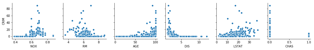
(a) For each predictor, fit a simple linear regression model to predict the response. Describe your results. In which of the models is there a statistically significant association between the predictor and the response? Create some plots to back up your assertions.
The p-values for $\beta_1$s suggest that for the model with predictor CHAS, we can not reject the null hypothesis and hence the model is not significant. The plots shown in the below figure suggest the same.
y = df_boston['CRIM']

X = df_boston[['ZN']]
X = sm.add_constant(X, prepend=True)
model = sm.OLS(y, X)
result = model.fit()
print(result.summary())
print("\n\n")

X = df_boston[['INDUS']]
X = sm.add_constant(X, prepend=True)
model = sm.OLS(y, X)
result = model.fit()
print(result.summary())
print("\n\n")

X = df_boston[['CHAS']]
X = sm.add_constant(X, prepend=True)
model = sm.OLS(y, X)
result = model.fit()
print(result.summary())
print("\n\n")

X = df_boston[['NOX']]
X = sm.add_constant(X, prepend=True)
model = sm.OLS(y, X)
result = model.fit()
print(result.summary())
print("\n\n")

X = df_boston[['RM']]
X = sm.add_constant(X, prepend=True)
model = sm.OLS(y, X)
result = model.fit()
print(result.summary())
print("\n\n")

X = df_boston[['AGE']]
X = sm.add_constant(X, prepend=True)
model = sm.OLS(y, X)
result = model.fit()
print(result.summary())
print("\n\n")

X = df_boston[['DIS']]
X = sm.add_constant(X, prepend=True)
model = sm.OLS(y, X)
result = model.fit()
print(result.summary())
print("\n\n")

X = df_boston[['RAD']]
X = sm.add_constant(X, prepend=True)
model = sm.OLS(y, X)
result = model.fit()
print(result.summary())
print("\n\n")

X = df_boston[['TAX']]
X = sm.add_constant(X, prepend=True)
model = sm.OLS(y, X)
result = model.fit()
print(result.summary())
print("\n\n")

X = df_boston[['PTRATIO']]
X = sm.add_constant(X, prepend=True)
model = sm.OLS(y, X)
result = model.fit()
print(result.summary())
print("\n\n")

X = df_boston[['B']]
X = sm.add_constant(X, prepend=True)
model = sm.OLS(y, X)
result = model.fit()
print(result.summary())
print("\n\n")

X = df_boston[['LSTAT']]
X = sm.add_constant(X, prepend=True)
model = sm.OLS(y, X)
result = model.fit()
print(result.summary())
print("\n\n")
OLS Regression Results
==============================================================================
Dep. Variable: CRIM R-squared: 0.040
Model: OLS Adj. R-squared: 0.038
Method: Least Squares F-statistic: 20.88
Date: Thu, 06 Sep 2018 Prob (F-statistic): 6.15e-06
Time: 21:37:49 Log-Likelihood: -1795.8
No. Observations: 506 AIC: 3596.
Df Residuals: 504 BIC: 3604.
Df Model: 1
Covariance Type: nonrobust
==============================================================================
coef std err t P>|t| [0.025 0.975]
------------------------------------------------------------------------------
const 4.4292 0.417 10.620 0.000 3.610 5.249
ZN -0.0735 0.016 -4.570 0.000 -0.105 -0.042
==============================================================================
Omnibus: 568.366 Durbin-Watson: 0.862
Prob(Omnibus): 0.000 Jarque-Bera (JB): 32952.356
Skew: 5.270 Prob(JB): 0.00
Kurtosis: 41.103 Cond. No. 28.8
==============================================================================
Warnings:
[1] Standard Errors assume that the covariance matrix of the errors is correctly specified.
OLS Regression Results
==============================================================================
Dep. Variable: CRIM R-squared: 0.164
Model: OLS Adj. R-squared: 0.162
Method: Least Squares F-statistic: 98.58
Date: Thu, 06 Sep 2018 Prob (F-statistic): 2.44e-21
Time: 21:37:49 Log-Likelihood: -1760.9
No. Observations: 506 AIC: 3526.
Df Residuals: 504 BIC: 3534.
Df Model: 1
Covariance Type: nonrobust
==============================================================================
coef std err t P>|t| [0.025 0.975]
------------------------------------------------------------------------------
const -2.0509 0.668 -3.072 0.002 -3.362 -0.739
INDUS 0.5068 0.051 9.929 0.000 0.407 0.607
==============================================================================
Omnibus: 585.528 Durbin-Watson: 0.990
Prob(Omnibus): 0.000 Jarque-Bera (JB): 41469.710
Skew: 5.456 Prob(JB): 0.00
Kurtosis: 45.987 Cond. No. 25.1
==============================================================================
Warnings:
[1] Standard Errors assume that the covariance matrix of the errors is correctly specified.
OLS Regression Results
==============================================================================
Dep. Variable: CRIM R-squared: 0.003
Model: OLS Adj. R-squared: 0.001
Method: Least Squares F-statistic: 1.546
Date: Thu, 06 Sep 2018 Prob (F-statistic): 0.214
Time: 21:37:49 Log-Likelihood: -1805.3
No. Observations: 506 AIC: 3615.
Df Residuals: 504 BIC: 3623.
Df Model: 1
Covariance Type: nonrobust
==============================================================================
coef std err t P>|t| [0.025 0.975]
------------------------------------------------------------------------------
const 3.7232 0.396 9.404 0.000 2.945 4.501
CHAS -1.8715 1.505 -1.243 0.214 -4.829 1.086
==============================================================================
Omnibus: 562.698 Durbin-Watson: 0.822
Prob(Omnibus): 0.000 Jarque-Bera (JB): 30864.755
Skew: 5.205 Prob(JB): 0.00
Kurtosis: 39.818 Cond. No. 3.96
==============================================================================
Warnings:
[1] Standard Errors assume that the covariance matrix of the errors is correctly specified.
OLS Regression Results
==============================================================================
Dep. Variable: CRIM R-squared: 0.174
Model: OLS Adj. R-squared: 0.173
Method: Least Squares F-statistic: 106.4
Date: Thu, 06 Sep 2018 Prob (F-statistic): 9.16e-23
Time: 21:37:50 Log-Likelihood: -1757.6
No. Observations: 506 AIC: 3519.
Df Residuals: 504 BIC: 3528.
Df Model: 1
Covariance Type: nonrobust
==============================================================================
coef std err t P>|t| [0.025 0.975]
------------------------------------------------------------------------------
const -13.5881 1.702 -7.986 0.000 -16.931 -10.245
NOX 30.9753 3.003 10.315 0.000 25.076 36.875
==============================================================================
Omnibus: 591.496 Durbin-Watson: 0.994
Prob(Omnibus): 0.000 Jarque-Bera (JB): 42994.381
Skew: 5.544 Prob(JB): 0.00
Kurtosis: 46.776 Cond. No. 11.3
==============================================================================
Warnings:
[1] Standard Errors assume that the covariance matrix of the errors is correctly specified.
OLS Regression Results
==============================================================================
Dep. Variable: CRIM R-squared: 0.048
Model: OLS Adj. R-squared: 0.046
Method: Least Squares F-statistic: 25.62
Date: Thu, 06 Sep 2018 Prob (F-statistic): 5.84e-07
Time: 21:37:50 Log-Likelihood: -1793.5
No. Observations: 506 AIC: 3591.
Df Residuals: 504 BIC: 3600.
Df Model: 1
Covariance Type: nonrobust
==============================================================================
coef std err t P>|t| [0.025 0.975]
------------------------------------------------------------------------------
const 20.5060 3.362 6.099 0.000 13.901 27.111
RM -2.6910 0.532 -5.062 0.000 -3.736 -1.646
==============================================================================
Omnibus: 576.890 Durbin-Watson: 0.883
Prob(Omnibus): 0.000 Jarque-Bera (JB): 36966.825
Skew: 5.361 Prob(JB): 0.00
Kurtosis: 43.477 Cond. No. 58.4
==============================================================================
Warnings:
[1] Standard Errors assume that the covariance matrix of the errors is correctly specified.
OLS Regression Results
==============================================================================
Dep. Variable: CRIM R-squared: 0.123
Model: OLS Adj. R-squared: 0.121
Method: Least Squares F-statistic: 70.72
Date: Thu, 06 Sep 2018 Prob (F-statistic): 4.26e-16
Time: 21:37:50 Log-Likelihood: -1772.9
No. Observations: 506 AIC: 3550.
Df Residuals: 504 BIC: 3558.
Df Model: 1
Covariance Type: nonrobust
==============================================================================
coef std err t P>|t| [0.025 0.975]
------------------------------------------------------------------------------
const -3.7527 0.944 -3.974 0.000 -5.608 -1.898
AGE 0.1071 0.013 8.409 0.000 0.082 0.132
==============================================================================
Omnibus: 575.090 Durbin-Watson: 0.960
Prob(Omnibus): 0.000 Jarque-Bera (JB): 36851.412
Skew: 5.331 Prob(JB): 0.00
Kurtosis: 43.426 Cond. No. 195.
==============================================================================
Warnings:
[1] Standard Errors assume that the covariance matrix of the errors is correctly specified.
OLS Regression Results
==============================================================================
Dep. Variable: CRIM R-squared: 0.143
Model: OLS Adj. R-squared: 0.141
Method: Least Squares F-statistic: 83.97
Date: Thu, 06 Sep 2018 Prob (F-statistic): 1.27e-18
Time: 21:37:50 Log-Likelihood: -1767.1
No. Observations: 506 AIC: 3538.
Df Residuals: 504 BIC: 3547.
Df Model: 1
Covariance Type: nonrobust
==============================================================================
coef std err t P>|t| [0.025 0.975]
------------------------------------------------------------------------------
const 9.4489 0.731 12.934 0.000 8.014 10.884
DIS -1.5428 0.168 -9.163 0.000 -1.874 -1.212
==============================================================================
Omnibus: 577.090 Durbin-Watson: 0.957
Prob(Omnibus): 0.000 Jarque-Bera (JB): 37542.100
Skew: 5.357 Prob(JB): 0.00
Kurtosis: 43.815 Cond. No. 9.32
==============================================================================
Warnings:
[1] Standard Errors assume that the covariance matrix of the errors is correctly specified.
OLS Regression Results
==============================================================================
Dep. Variable: CRIM R-squared: 0.387
Model: OLS Adj. R-squared: 0.386
Method: Least Squares F-statistic: 318.1
Date: Thu, 06 Sep 2018 Prob (F-statistic): 1.62e-55
Time: 21:37:50 Log-Likelihood: -1682.3
No. Observations: 506 AIC: 3369.
Df Residuals: 504 BIC: 3377.
Df Model: 1
Covariance Type: nonrobust
==============================================================================
coef std err t P>|t| [0.025 0.975]
------------------------------------------------------------------------------
const -2.2709 0.445 -5.105 0.000 -3.145 -1.397
RAD 0.6141 0.034 17.835 0.000 0.546 0.682
==============================================================================
Omnibus: 654.232 Durbin-Watson: 1.336
Prob(Omnibus): 0.000 Jarque-Bera (JB): 74327.568
Skew: 6.441 Prob(JB): 0.00
Kurtosis: 60.961 Cond. No. 19.2
==============================================================================
Warnings:
[1] Standard Errors assume that the covariance matrix of the errors is correctly specified.
OLS Regression Results
==============================================================================
Dep. Variable: CRIM R-squared: 0.336
Model: OLS Adj. R-squared: 0.335
Method: Least Squares F-statistic: 254.9
Date: Thu, 06 Sep 2018 Prob (F-statistic): 9.76e-47
Time: 21:37:50 Log-Likelihood: -1702.5
No. Observations: 506 AIC: 3409.
Df Residuals: 504 BIC: 3418.
Df Model: 1
Covariance Type: nonrobust
==============================================================================
coef std err t P>|t| [0.025 0.975]
------------------------------------------------------------------------------
const -8.4748 0.818 -10.365 0.000 -10.081 -6.868
TAX 0.0296 0.002 15.966 0.000 0.026 0.033
==============================================================================
Omnibus: 634.003 Durbin-Watson: 1.252
Prob(Omnibus): 0.000 Jarque-Bera (JB): 63141.063
Skew: 6.134 Prob(JB): 0.00
Kurtosis: 56.332 Cond. No. 1.16e+03
==============================================================================
Warnings:
[1] Standard Errors assume that the covariance matrix of the errors is correctly specified.
[2] The condition number is large, 1.16e+03. This might indicate that there are
strong multicollinearity or other numerical problems.
OLS Regression Results
==============================================================================
Dep. Variable: CRIM R-squared: 0.083
Model: OLS Adj. R-squared: 0.081
Method: Least Squares F-statistic: 45.67
Date: Thu, 06 Sep 2018 Prob (F-statistic): 3.88e-11
Time: 21:37:50 Log-Likelihood: -1784.1
No. Observations: 506 AIC: 3572.
Df Residuals: 504 BIC: 3581.
Df Model: 1
Covariance Type: nonrobust
==============================================================================
coef std err t P>|t| [0.025 0.975]
------------------------------------------------------------------------------
const -17.5307 3.147 -5.570 0.000 -23.714 -11.347
PTRATIO 1.1446 0.169 6.758 0.000 0.812 1.477
==============================================================================
Omnibus: 568.808 Durbin-Watson: 0.909
Prob(Omnibus): 0.000 Jarque-Bera (JB): 34373.378
Skew: 5.256 Prob(JB): 0.00
Kurtosis: 41.985 Cond. No. 160.
==============================================================================
Warnings:
[1] Standard Errors assume that the covariance matrix of the errors is correctly specified.
OLS Regression Results
==============================================================================
Dep. Variable: CRIM R-squared: 0.142
Model: OLS Adj. R-squared: 0.141
Method: Least Squares F-statistic: 83.69
Date: Thu, 06 Sep 2018 Prob (F-statistic): 1.43e-18
Time: 21:37:50 Log-Likelihood: -1767.2
No. Observations: 506 AIC: 3538.
Df Residuals: 504 BIC: 3547.
Df Model: 1
Covariance Type: nonrobust
==============================================================================
coef std err t P>|t| [0.025 0.975]
------------------------------------------------------------------------------
const 16.2680 1.430 11.376 0.000 13.458 19.078
B -0.0355 0.004 -9.148 0.000 -0.043 -0.028
==============================================================================
Omnibus: 591.626 Durbin-Watson: 1.001
Prob(Omnibus): 0.000 Jarque-Bera (JB): 43282.465
Skew: 5.543 Prob(JB): 0.00
Kurtosis: 46.932 Cond. No. 1.49e+03
==============================================================================
Warnings:
[1] Standard Errors assume that the covariance matrix of the errors is correctly specified.
[2] The condition number is large, 1.49e+03. This might indicate that there are
strong multicollinearity or other numerical problems.
OLS Regression Results
==============================================================================
Dep. Variable: CRIM R-squared: 0.205
Model: OLS Adj. R-squared: 0.203
Method: Least Squares F-statistic: 129.6
Date: Thu, 06 Sep 2018 Prob (F-statistic): 7.12e-27
Time: 21:37:50 Log-Likelihood: -1748.2
No. Observations: 506 AIC: 3500.
Df Residuals: 504 BIC: 3509.
Df Model: 1
Covariance Type: nonrobust
==============================================================================
coef std err t P>|t| [0.025 0.975]
------------------------------------------------------------------------------
const -3.2946 0.695 -4.742 0.000 -4.660 -1.930
LSTAT 0.5444 0.048 11.383 0.000 0.450 0.638
==============================================================================
Omnibus: 600.766 Durbin-Watson: 1.184
Prob(Omnibus): 0.000 Jarque-Bera (JB): 49637.173
Skew: 5.638 Prob(JB): 0.00
Kurtosis: 50.193 Cond. No. 29.7
==============================================================================
Warnings:
[1] Standard Errors assume that the covariance matrix of the errors is correctly specified.
sns.pairplot(df_boston, y_vars=['CRIM'], x_vars=['NOX', 'RM', 'AGE', 'DIS', 'LSTAT', 'CHAS'])
<seaborn.axisgrid.PairGrid at 0x11bb509e8>
(b) Fit a multiple regression model to predict the response using all of the predictors. Describe your results. For which predictors can we reject the null hypothesis H0 : βj = 0?
For the predictors: DIS, RAD, BLACK, LSTAT, we can reject the null hypothesis.
Y = df_boston['CRIM']
X = df_boston[['ZN', 'INDUS', 'CHAS', 'NOX', 'RM', 'AGE', 'DIS', 'RAD', 'TAX', 'PTRATIO', 'B', 'LSTAT']]
X = sm.add_constant(X, prepend=True)
model = sm.OLS(y, X)
result = model.fit()
print(result.summary())
                            OLS Regression Results
==============================================================================
Dep. Variable:                   CRIM   R-squared:                       0.436
Model:                            OLS   Adj. R-squared:                  0.422
Method:                 Least Squares   F-statistic:                     31.77
Date:                Thu, 06 Sep 2018   Prob (F-statistic):           6.16e-54
Time:                        21:37:50   Log-Likelihood:                -1661.2
No. Observations:                 506   AIC:                             3348.
Df Residuals:                     493   BIC:                             3403.
Df Model:                          12
Covariance Type:            nonrobust
==============================================================================
                 coef    std err          t      P>|t|      [0.025      0.975]
------------------------------------------------------------------------------
const         10.3701      7.012      1.479      0.140      -3.408      24.148
ZN             0.0365      0.019      1.936      0.053      -0.001       0.073
INDUS         -0.0672      0.085     -0.794      0.428      -0.233       0.099
CHAS          -1.3049      1.185     -1.101      0.271      -3.633       1.023
NOX           -7.2552      5.250     -1.382      0.168     -17.570       3.060
RM            -0.3851      0.575     -0.670      0.503      -1.515       0.745
AGE            0.0019      0.018      0.105      0.917      -0.034       0.038
DIS           -0.7163      0.273     -2.626      0.009      -1.252      -0.180
RAD            0.5395      0.088      6.128      0.000       0.366       0.712
TAX           -0.0013      0.005     -0.254      0.799      -0.011       0.009
PTRATIO       -0.0907      0.180     -0.504      0.615      -0.445       0.263
B             -0.0089      0.004     -2.428      0.016      -0.016      -0.002
LSTAT          0.2309      0.069      3.346      0.001       0.095       0.366
==============================================================================
Omnibus:                      680.813   Durbin-Watson:                   1.507
Prob(Omnibus):                  0.000   Jarque-Bera (JB):            94712.935
Skew:                           6.846   Prob(JB):                         0.00
Kurtosis:                      68.611   Cond. No.                     1.51e+04
==============================================================================

Warnings:
[1] Standard Errors assume that the covariance matrix of the errors is correctly specified.
[2] The condition number is large, 1.51e+04. This might indicate that there are
strong multicollinearity or other numerical problems.