Classification
A process for predicting qualitative or categorical variables is called as Classification.
4.1 An Overview of Classification
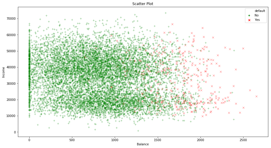
The dataset used in this chapter will be Default dataset. We will predict that whether an individual will default on his/her credit card payment on the basis of annual income and monthly credit card balance. The data is displayed below:
import pandas as pd
import seaborn as sns
import matplotlib.pyplot as plt
default = pd.read_excel("data/Default.xlsx")
markers = {"Yes": "x", "No": "+"}
palette = {"Yes": "red", "No": "green"}
fig = plt.figure(figsize=(15,8))
ax = fig.add_subplot(111)
sns.scatterplot(x="balance", y="income", hue="default", style="default", markers=markers, palette=palette,
alpha=0.6, data=default)
ax.set_xlabel('Balance')
ax.set_ylabel('Income')
ax.set_title('Scatter Plot')
fig = plt.figure(figsize=(15,8))
ax = fig.add_subplot(121)
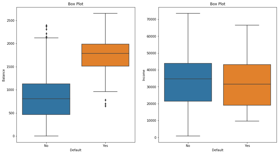
sns.boxplot(x="default", y="balance", data=default)
ax.set_xlabel('Default')
ax.set_ylabel('Balance')
ax.set_title('Box Plot')
ax = fig.add_subplot(122)
sns.boxplot(x="default", y="income", data=default)
ax.set_xlabel('Default')
ax.set_ylabel('Income')
ax.set_title('Box Plot')
plt.show()
4.2 Why Not Linear Regression?
In general, there is no natural way to convert a qualitative response variable with more than two levels into a quantitative response that is ready for linear regression. For the binary qualitative response, we can simply encode the variables as 0 and 1 and predict the values taking 0.5 as threshold.
4.3 Logistic Regression
Rather than modeling the response directly, logistic regression models the probability that response $Y$ belongs to a particular category. For the Default data, logistic regression models the probability of default. The probability of default given balance can be written as $Pr \ (default=Yes \ | \ balance)$, and can be abbreviated as $p(balance)$. We can choose a threshold and then predict default as Yes if $p(balance) > 0.5$. If we want to be more conservative, we can lower the threshold.
4.3.1 The Logistic Model
The problem with using linear regression to predict a qualitative variable is that any time a straight line is fit to a binary response that is coded as 0 and 1, in principle we can always predict $p(X) < 0$ and $p(X) > 1$ for some values of X. To avoid this problem, we can use a function instead that gives output between 0 and 1 for all values of X. In logistic regression we use logistic function, which is given as:
$$p(X) = \frac{e^{\beta_0 + \beta_1X}}{1 + e^{\beta_0 + \beta_1X}}$$
and to fit the model, we can use maximum likelihood. The logistic function produces a S-shaped curve. Manipulating the above equation, we get:
$$\frac{p(X)}{1 - p(X)} = e^{\beta_0 + \beta_1X}$$
The quantity on the left hand side is called as odds and can take any value between 0 and $\infty$. A lower and higher value of odds suggest a very low and high probabilities of default respectively. By taking the logarithm of both sides, we get:
$$log \bigg( \frac{p(X)}{1 - p(X)} \bigg) = \beta_0 + \beta_1X$$
The left hand side of above equation is called log-odds or logit. For a logistic regression model, logit is linear in X. The interpretation is as follows: For a one unit increase in X, the logit increases by $\beta_1$, or odds is multiplied by $e^{\beta_1}$.
The amount that $p(X)$ changes due to one unit change in X, depends on current value of X. If $\beta_1$ is positive, increasing X is associated with increasing $p(X)$. If $\beta_1$ is negative, increasing X is associated with decreasing $p(X)$.
4.3.2 Estimating the Regression Coefficients
Non-linear least squares can be used to fit the logistic regression model but a more general method of maximum-likelihood is preferred as it has better statistical properties. In maximum-likelihood, we seek estimates of $\beta_0$ and $\beta_1$ such that the predicted probabilities corresponds as closely as possible to the observed individual probabilities. In the case of the prediction of default status, by plugging in the values of $\beta$s in the model, we should get value of $p(X)$ for default as Yes close to 1 and for No, close to 0. This intution can be formalized using a mathematical equation called as likelihood function:
$$l(\beta_0, \beta_1) = \prod _{i:y_i = 1} p(x_i) \prod _{i^{’}:y _{i^{’}} = 0} (1 - p(x _{i^{’}}))$$
The estimates are chosen to maximize this function. Maximum likelihood is a very general approach that can be used to fit many of the non-linear models.
In the logistic regression output, we can verify the statistical signifance of the model the same way as for the linear regression output. Instead of t-statistic, we use z-statistic which is defined the same ($\widehat{\beta_1} \ / \ SE(\widehat{\beta_1})$). The null hypothesis implies that $\beta_1 = 0$, i.e. $p(X) = \frac{e^{\beta_0}}{1 + e^{\beta_0}}$, which means the probability of default does not depend on balance. The main purpose of the intercept is to adjust the average fitted probability to the proportion of ones in the data.
4.3.3 Making Predictions
The prediction step is similar to the linear regression as well. Qualitative variables can be used in the similar manner as the linear regression.
4.3.4 Multiple Logistic Regression
Multiple logistic regression can be modeled as:
$$p(X) = \frac{e^{\beta_0 + \beta_1X_1 + … + \beta_pX_p}}{1 + e^{\beta_0 + \beta_1X_1 + … + \beta_pX_p}}$$
$$log \bigg( \frac{p(X)}{1-p(X)} \bigg) = \beta_0 + \beta_1X_1 + … + \beta_pX_p$$
Confounding is a phenomenon which explains the errors associated with logistic regression when results obtained using one predictor is quite different than the one using multiple predictors, especially when there is a correlation among the predictors.
4.3.5 Logistic Regression for >2 Response Classes
Multi-class logistic regression is not used much. Instead, discriminant analysis is popular for multi-class classification.