3.7 Exercises
Conceptual
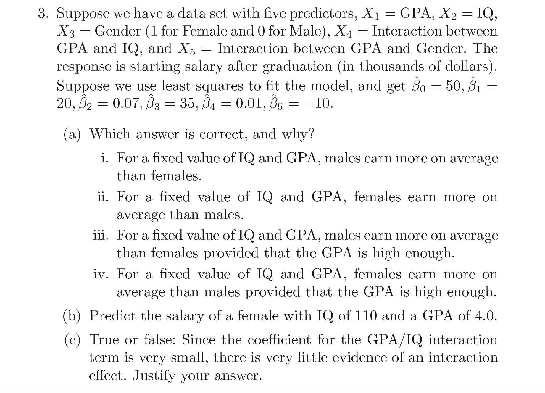
Solution: The linear fit can be given as:
$$50 + (20 \times GPA) + (0.07 \times IQ) + (35 \times GENDER) + (0.01 \times GPA \times IQ) - (10 \times GPA \times GENDER)$$
(a) For a fixed value of IQ and GPA, the average salary for male will be $50 + 20 \times GPA$ and for the female it will be $85 + 20 \times GPA - 10 \times GPA$. For the salary of male to be higher, $50 + 20GPA > 85 + 10GPA$, i.e. $GPA > 3.5$.
Hence, the true statement is: For a fixed value of IQ and GPA, males earn more on average than females provided that the GPA is high enough.
(b) The prediction is 137.1 and hence the salary will be $137100.
(c) False. We need to test the hypothesis for the coefficient to be equal to 0.
Solution 4: (a) As the true relationship between $X$ and $Y$ is linear, there is a chance that the RSS of training data for the linear model will be lower. But as the RSS highly depends on the distribution of points, there is a chance that the polynomial regression can overfit the points and hence can results in lower RSS.
(b) Test RSS for the linear model should be lower as the test data should follow the linear curve.
(c) The polynomial regression, being the more flexible one will follow the training data more closely and hence resulting in lower training RSS.
(d) For the test data, we can not conclude anything without observing the data.
Solution 5: $a_i^{’}$ can be calculated as:
$$a_i^{’} = \frac{x_i x_i^{’}}{\sum _{k=1}^{n}x_k^2}$$
Solution 6: The least square line can be denoted as:
$$y = \widehat{\beta_0} + \widehat{\beta_1}x$$
Substituting $\bar{x}$ and replacing the optimal value of $\beta_0$, we get:
$$y = \widehat{\beta_0} + \widehat{\beta_1}\bar{x} = (\bar{y} - \widehat{\beta_1}\bar{x}) + \widehat{\beta_1}\bar{x} = \bar{y}$$
Solution 7: Assumption: $\bar{x} = 0, \bar{y} = 0$. The correlation is given as:
$$r = \frac{\sum _{i=1}^{n}(x_i - \bar{x})(y_i - \bar{y})}{\sqrt{\sum _{i=1}^{n} (x_i - \bar{x})^2} \sqrt{\sum _{i=1}^{n} (y_i - \bar{y})^2}} = \frac{\sum _{i=1}^{n}(x_i)(y_i)}{\sqrt{\sum _{i=1}^{n} (x_i)^2} \sqrt{\sum _{i=1}^{n} (y_i)^2}}$$
R-statistic is given as (Replacing $\bar{y} = 0, \beta_0 = 0$):
$$R^2 = 1 - \frac{RSS}{TSS} = 1 - \frac{\sum _{i=1}^{n} (\widehat{y_i} - y_i)^2}{\sum _{i=1}^{n} (y_i - \bar{y})^2} = 1 - \frac{\sum _{i=1}^{n} (\widehat{y_i} - y_i)^2}{\sum _{i=1}^{n} (y_i)^2} = 1 - \frac{\sum _{i=1}^{n}(\beta_0 + \beta_1 x_i - y_i)^2}{\sum _{i=1}^{n} (y_i)^2} = 1 - \frac{\sum _{i=1}^{n} (\beta_1 x_i - y_i)^2}{\sum _{i=1}^{n} (y_i)^2}$$
$\beta_1$ is given as:
$$\beta_1 = \frac{\sum _{i=1}^{n} (x_i - \bar{x}) (y_i - \bar{y})}{\sum _{i=1}^{n}(x_i - \bar{x})^2} = \frac{\sum _{i=1}^{n} x_i y_i}{\sum _{i=1}^{n}(x_i)^2}$$
Replacing $\beta_1$ in the above equation and solving we get,
$$R^2 = \frac{\sum_i (y_i)^2 - (\sum_i (y_i)^2 + \sum_i (\beta_1x_i)^2 - \sum_i{2\beta_1 x_i y_i})}{\sum_i (y_i)^2} = \frac{\sum_i{2\beta_1 x_i y_i} - \sum_i (\beta_1x_i)^2}{\sum_i (y_i)^2} = r^2$$