3.3 Other Considerations in the Regression Model
3.3.1 Qualitative Predictors
There can be a case when predictor variables can be qualitative.
Predictors with Only Two Levels
For the predictors with only two values, we can create an indicator or dummy variable with values 0 and 1 and use it in the regression model. The final prediction will not depend on the coding scheme. Only difference will be in the model coefficients and the way they are interpreted.
Qualitative Predictors with More than Two Levels
When a qualitative predictor has more than two levels, we can use more than one single dummy variable to encode them. There will always be one less dummy variable than the number of levels.
3.3.2 Extensions of the Linear Model
Standard linear regression provides results that work quite well on real world problems. However, it makes two restrictive assumptions:
-
Additive: Relationship between response and predictor is additive, which means that the effect of change in the predictor $X_i$ on the response $Y$ is independent of the values of other predictors.
-
Linear: Change in response $Y$ due to one unit change in $X_j$ is constant.
Removing the Additive Assumption
A synergy or an interaction effect is described as the phenomenon when two predictors can interact while deciding on response. Linear model can be extended and take into account an interaction term($X_1X_2$) as follows:
$$Y = \beta_0 + \beta_1X_1 + \beta_2X_2 + \beta_3X_1X_2 + \epsilon$$
There may be a case when interaction term has a very small p-value but the associated main effects do not. The hierarchial principal states that if we include the interaction term in the model, we should also include the main effect, even if the associated p-values are not significant.
Interaction effect of qualitative with quantitative variables can be incorporated in the same way.
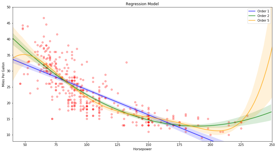
Non-linear Relationships
Polynomial Regression can be used to extend the linear model to accomodate the non-linear relationship. The various regression models for miles per gallon vs horsepower for auto data is shown below. A simple way to incorporate non-linear associations in a linear model is by adding transformed versions of the predictors as follows (order 2):
$$mpg = \beta_0 + \beta_1 \times horsepower + \beta_2 \times horsepower^2 + \epsilon $$
This approach is called as polynomial regression.
auto = pd.read_csv("data/Auto.csv")
auto.dropna(inplace=True)
auto = auto[auto['horsepower'] != '?']
auto['horsepower'] = auto['horsepower'].astype(int)

fig = plt.figure(figsize=(15,8))
ax = fig.add_subplot(111)
sns.regplot(x="horsepower", y="mpg", color='r', fit_reg=True, data=auto, order=1, scatter_kws={'alpha':0.1},
            line_kws={'color':'blue', 'alpha':0.7, 'label':'Order 1'})
sns.regplot(x="horsepower", y="mpg", color='r', fit_reg=True, data=auto, order=2, scatter_kws={'alpha':0.1},
            line_kws={'color':'g', 'alpha':0.7, 'label':'Order 2'})
sns.regplot(x="horsepower", y="mpg", color='r', fit_reg=True, data=auto, order=5, scatter_kws={'alpha':0.1},
            line_kws={'color':'orange', 'alpha':0.7, 'label':'Order 5'})

ax.set_xlabel('Horsepower')
ax.set_ylabel('Miles Per Gallon')
ax.set_title('Regression Model')
ax.set_ylim(8, 50)
ax.set_xlim(40, 250)
ax.legend()

plt.show()
/Users/amitrajan/Desktop/PythonVirtualEnv/Python3_VirtualEnv/lib/python3.6/site-packages/scipy/stats/stats.py:1713: FutureWarning: Using a non-tuple sequence for multidimensional indexing is deprecated; use `arr[tuple(seq)]` instead of `arr[seq]`. In the future this will be interpreted as an array index, `arr[np.array(seq)]`, which will result either in an error or a different result.
  return np.add.reduce(sorted[indexer] * weights, axis=axis) / sumval
3.3.3 Potential Problems
The problems which arise when we fit a linear regression to a particular data set are as follows:
-
Non-linearity of the Data:
Residual plots are a useful graphical tool for identifying non-linearity. For simple linear regression, a plot of residual vd predictor can be analyzed. In the case of multiple linear regression, as there are multiple predictors, a plot of residuals vs predicted values can be analyzed. Ideally, the residual plot will show no discernible pattern. The presence of a pattern may indicate a problem with some aspect of the linear model. If the residual plots indicate that there is a non-linear associations in the data, non-linear transformation of the predictors can be used in the model.
-
Correlation of Error Terms:
An important assumption of linear regression model is that the error terms are uncorrelated. If there is a correlation between the error terms, the estimated standard errors will tend to underestimate the true standard errors. As a result, the confidence and prediction intervals will be narrower and the p-value associated with the model will be lower which results in an unwarranted sense of confidence in the model.d
Correlation in error terms might occur in the context of time series data. This can be visualized by plotting the residuals against time and checking for a discernable pattern.
-
Non-constant Variance of Error Terms:
Another assumption of the linear regression model is that the error terms have a constant variance. The non-constant variances in the errors can be identified by the presence of a funnel shape in the residual plot. When faced with this problem one possible approach is to transform the response $Y$ using a concave function $logY$ or $\sqrt Y$.
-
Outliers:
An outlier may have a little effect on the least square fit but it can cause other problems like high value of RSE and lower R$^2$ values which can affect the interpretation of the model. Residual plots can be used to identify outliers.
-
High Leverage Points:
High leverage points have an unsual values for $x_i$. Removing high leverage point has more substantial impact on the least square line compared to the outliers. Hence it is important to identify high leverage points. In a simple linear regression, it is easy to check on the range of the predictors and find the high levarage points. For a multiple linear regression, the predictors may lie in their individual ranges but can lie outside in terms of the full set of predictors. Leverage statistic is a way to identify the high leverage points. A large value of this statistic indicates high leverage.
-
Collinearity:
When two or more predictor variables are closely related to each other, a situation of collinearity arises. Due to collinearity, it can be impossible to separate out the individual effects of collinear variables on the response. Collinearity also reduces the estimation accuracy of the regression coefficients. As t-statistic of a predictor is calculated by dividing $\beta_i$ by its standard error, and hence collinearity results in the decline of t-statistic and consequently we may fail to reject the null hypothesis.
A simple approach is to detect collinearity is by analyzing the correlation matrix. This process has a drawback as it can not detect multicollinearity (collinearity between three or more variables). A better way to assess multicollinearity is by computing variance inflation factor (VIF). VIF is the ratio of variance in a model with multiple predictors, divided by the variance of a model with one predictor alone. Smallest possible value of VIF is 1 and as a rule of thumb, a VIF value that exceeds 5 or 10 indicates a problematic amount of collinearity.
There are two approaches to deal with the problem of collinearity. One is to simply drop one of the problematic variable. Alternatively we can combine the collinear variables together as a single predictor.
3.5 Comparison of Linear Regression with K-Nearest Neighbors
Linear regression is an example of parametric approach, as it assumes a linear form for $f(X)$. It has the advantage of easy to fit as we only need to estimate a small number of coefficients. The one disadvantage of parametric method is that, they make a strong assumption about the shape of $f(X)$ and hence can affect the prediction accuracy if the shape deviates from the assumption.
Non-parametric methods does not assume a parametric form for $f(X)$ and hence provide a more flexible approach for regression. KNN (K-nearest neighbors) regression is an example of this.
KNN regression first identifies $K$ nearest training observations to $x_0$, represented as $N_0$. It then estimates $f(x_0)$ as the average of the training responses in $N_0$ as:
$$\widehat{f}(x_0) = \frac{1}{K} \sum _{x_i \in N_0} y_i$$
As the value of $K$ increases, the smothness of fit increases. The optimal vale of $K$ depends on the bias-variance tradeoff. A small value of $K$ provides the most flexible fit, which will have low bias but high variance. On contrast larger value of $K$ provides a smoother and less variable fit (as prediction depends on more points, changing one will have smaller effect on the overall prediction).
The parametric approach will outperform the nonparametric approach if the parametric form that has been selected is close to the true form of $f$. In this case, the non-parametric approach incurs a cost in variance that is not offset by a reduction in bias. As level of non-linearlity increases, for $p=1$, KNN regression outperforms linear regression. But as number of predictors increases, the performance of linear regression is better than KNN. This arises due to the phenomenon which can be termed as curse of dimensionality. As the number of predictors increase, number of dimensions increases and hence the given test observation $x_0$ may be very far away in the p-dimensional space when p is large and hence a poor KNN fit. As a general rule, parametric methods will tend to outperform non-parametric approaches when there is a small number of observations per predictor. Even when the dimension is small, linear regression is preferred due to better interpretability.