The one assumption for the Student’s t tests performed above was the fact that the samples should come from the normal distribution. In distribution-free tests, this restriction is relaxed, i.e. the samnples are not required to come from any specific distribution. Distribution-free tests are sometimes called as nonparametric tests. Mainly, there are two types of distribution-free tests: Wilcoxon signed-rank test(test for population mean) and Wilcoxon rank-sum test / Mann-Whitney test (analogous to the two-sample t test).
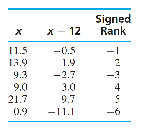
#### The Wilcoxon Signed-Rank Test :Let us see an example to understand the Wilcoxon signed-rank test. Below table shows the measurement of a quantity in a particular experiment. A test for $H_0: \mu \geq 12$ against $H_A: \mu < 12$ needs to be conducted. From the data set, it can be seen that it contains two outliers as 0.9 and 21.7 and hence the samples do not come from normal population. This makes the Student’s t test inappropriate.

The Wilcoxon Signed-Rank test does not require the population to be normal. Instead, it requires that the population has a continuous and symmetric probability density function. As the outliers are present on both sides, we can assume that the population is continuous and symmetric. As the population is symmetric, the median will be same as the mean. The next step is to make the data points median-centered. As, $\mu = 12$, the median will also be 12, we subtract 12 from each observation. Next, we find the rank (ignoring the signs) of median-centered observation, giving the rank 1 to the point which is closest to the median. Then the ranks are given the same sign as the one for the meadian-centered observations. Now, we calculate the sum of the positive and negative ranks as: $S+ = 2+5 = 7$ and S- = 1 + 3 + 4 + 6 = 14. Using simple mathematics, it can be shon that $(S+) + (S-) = \frac{n(n+1)}{2}$, where $n$ is the sample size. Hence, for a larger sample size, instead of finding both the sums, we can find one of the sums and can compute the another one as $S+ = n(n+1)/2 - S-$.
When, $\mu > 12$, the positive ranks are more probable than the negative ranks and tend to be larger in the magnitude as well, i.e. S_+ is likely to be large. If $\mu < 12$, the situation is reversed and hence the positive ranks are likely to be fewer in number and smaller in magnitude, so S_+ is likely to be small. Hence, in a nut shell, large value of $S_+$ will provide evidence against a null hypothesis of the form $H _0: \mu \leq \mu_0$ while smaller values of $S+$ will provide evidence against a null hypothesis of the form $H _0: \mu \geq \mu_0$. Here $S+$ is smaller and hence it gives the evidence against the null hypothesis which is $H_0: \mu \geq 12$. The p-value for the test can be calculated from the table as well as through various scientific packages.
One major hurdle while assigning the ranks is the case when a tie occurs. In this case, an average of the ranks is assigned to both the observations. For example, if there is a tie for the third and fourth rank, a rank of 3.5 is assigned to both the observations. Another cocern is the case when one of the observation is exactly equal to median (or mean). In this case, the difference will be 0 and the observation can not be assigned a rank. One way to deal with this is to drop this observation.
When the sample size is large, the test statistic $S+$ is approximately normally distributed with mean $n(n+1)/4$ and standard deviation $n(n+1)(2n+1)/24$. In this case, the Wilcoxon signed-rank test can be performed by computing the z-score of $S+$ and then the normal table can be used to find the p-value. The z-score is:
$$z = \frac{(S+) - n(n+1)/4}{\sqrt{n(n+1)(2n+1)/24}}$$
#### The Wilcoxon Rank-Sum Test :The Wilcoxon rank-sum test can be used to test the difference in population mean in the case when populations are not normal. It makes two assumptions: the populations must be continuous and their probability density functions must be identical in shape and size (location does not matter).
Let the random samples from two different populations be $X_1, X_2, …, X_m$ and $Y_1, Y_2, …, Y_n$ and the population means be $\mu_X$ and $\mu_Y$. The Wilcoxon rank-sum test is performed by combining the two samples and assigning a rank of $1, 2, …, m+n$ to them. The test statistic, $W$, is the sum of the ranks of the samples from $X$ (where $m \leq n$). As the populations are identical apart from the location, if $\mu_X < \mu_Y$, the sum of the rank of the observations from population $X$, which is the test statistic, will be smaller. If $\mu_X > \mu_Y$, $W$ will tend to be larger.
Let us look at an example. Following code performs a two-tailed Wilcoxon rank-sum on the samples from two populations $X$ and $Y$. For a one-tailed test, such as: $H_0: \mu_X \geq \mu_Y$ against $H_A: \mu_X < \mu_Y$, the p-value will be the half of the two-tailed test, which is 0.0223.
from scipy.stats import ranksums

X = [36, 28, 29, 20, 38]
Y = [34, 41, 35, 47, 49, 46]

print(ranksums(X, Y))
RanksumsResult(statistic=-2.008316044185609, pvalue=0.044609718024939606)
For a larger sample size ($m, n > 8$), it can be shown that the null disribution of test statistic $W$ is approximately normal with mean $\mu = m(m+n+1 /2)$ and variance $\sigma^2 = mn(m+n+1)/12$. In this case, we can compute the z-score of $W$ and a z-test can be performed. The test statistic is given as:
$$z = \frac{W - m(m+n+1 /2)}{\sqrt{mn(m+n+1)/12}}$$
There is a widespread misconception that distribution-free test methods are restriction free. Befor applying the distribution-free methods, one should always remember the restrictions of symmetry for the signed-rank test and of identical shape and size for rank-sum test.
### Reference :https://www.mheducation.com/highered/product/statistics-engineers-scientists-navidi/M0073401331.html