A generalization of the Bernoulli trial is the multinomial trial, which is an experiment that can rsult in any one of the $k$ outcomes where $k \geq 2$. Let the probabilities of the $k$ outcomes be denoted by $p_1, p_2, p_3, …, p_k$ and the prespecified values be $p _{01}, p _{02}, …, p _{0k}$. We need to conduct a test to chek whether the probabilities are equal to the prespecified values or not. The null hypothesis will be
$$H_0: p_1 = p _{01}, p_2 = p _{02}, …, p_k = p _{0k}$$
Suppose we want to test that whether a die is fair or not (i.e. we need to check that whether the probability of getting each outcome is $\frac{1}{6}$ or not). We conducted an ecperiment and rolled a die $600$ times. The outcomes are shown below.
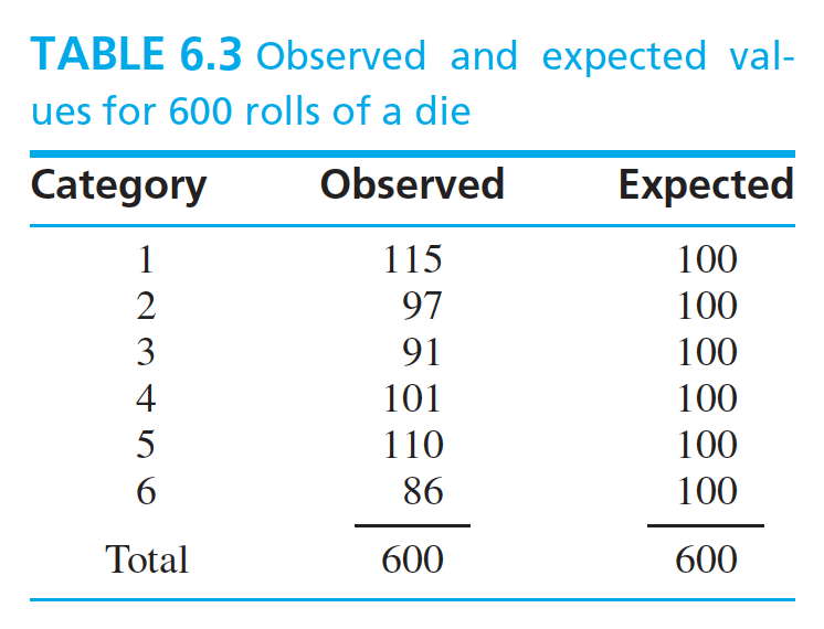
The results consist of observed and expected values. Observed values is the result of the experiment and expected values are calculated form the desired probabilities for a fair die. We need to test that whether the observed and expected values are close to each other or not i.e. we need to conduct a test for variance. Hence, the statistic used is called as chi-square statistic and is given as:
$$\chi^2 = \sum_{i=1}^{k}\frac{(O_i - E_i)^2}{E_i}$$
The larger the value of the test statistic, the farther the observed values from the expected values and hence the stronger the evidence against the null hypothesis $H_0$. To determine the p-value for the test, we need to find the distribution for the test statistic. For sufficiently large expected values, the test statistic follows the chi-square distribution with $k-1$ degrees of freedom. The test statistic for the given experiment is $\chi^2 = 6.12$ and it’s degree of freedom is $5$. From chi-square distribution, the upper 10% point is 9.236 and hence we can conclude that $p-value > 0.10$. We can not reject the null hypothesis then saying that there is no evidence that the die is not fair. The test described above determines that how well a given multinomial distribution fits the data and hence is also called as goodness-off-fit test.
### The Chi-Square Test for Homogeneity :Let us look at an example to understand the meaning of the test of homogeneity. Four machines manufacture cylindrical steel pins. The pins are subjected to a diameter specification. A pin may meet the specification, or it may be too thin or too thick. The results of the experiment is shown below.
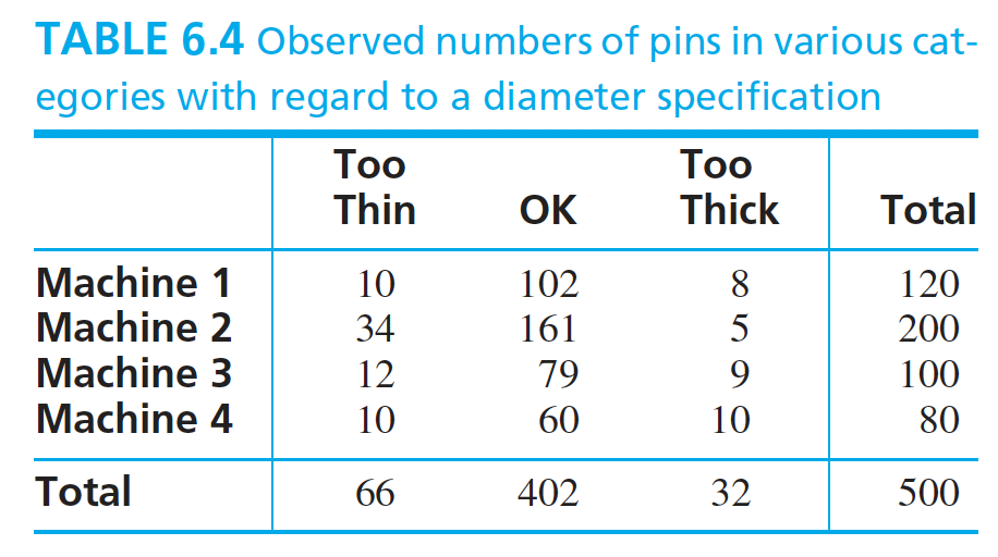
The above table is called as a contigency table. For the mentioned experiment, the null hypothesis is that the proportions of pins that are too thin, OK, or too thick is same for all the machines. Let $I$ denotes the number of rows in the table and $J$ denotes the number of columns. Let $p_{ij}$ denotes the probability of the outcome in the cell $(i, j)$. The the null hypothesis can be given as:
$$H_0: For \ ecah \ column \ j,\ p _{1j} = p _{2j} = … = p _{Ij}$$
Let $O_ {ij}$ denotes the observed value in the cell $(i, j)$, $O_ {i.}$ the sum of the observed values in the row $i$, $O_ {.j}$ the sum of the observed values in the column $j$ and $O_{..}$ the sum of observed values in all the cells. To calculate the test statistic, we need to find the expected values for the number of observations in each of the cells. This can be calculated as:
$$E_ {ij} = \frac{O_ {i.}O_ {.j}}{O_ {..}}$$
The test statistic is given as:
$$\chi^2 = \sum _{i=1}^{I} \sum _{j=1}^{J} \frac{(O _{ij} - E _{ij})^2}{E _{ij}}$$
Under null hypothesis, the test statistic has a chi-square distribution with $(I-1)(J-1)$ degrees of freedom. The test results for the above mentioned experiment is shown below.
import numpy as np
from scipy.stats import chi2_contingency

obs = np.array([[10, 102, 8], [34, 161, 5], [12, 79, 9], [10, 60, 10]])
chi2, p, dof, ex = chi2_contingency(obs, correction=False)
print("The expected values are: \n" + str(ex))
print("The degree of freedom is: " + str(dof))
print("The test statistic is: " + str(chi2))
print("The p-value is: " + str(p))
The expected values are:
[[ 15.84  96.48   7.68]
 [ 26.4  160.8   12.8 ]
 [ 13.2   80.4    6.4 ]
 [ 10.56  64.32   5.12]]
The degree of freedom is: 6
The test statistic is: 15.584353328056686
The p-value is: 0.01616760116149423
In the above experiment, the row totals (the number of pins manufactured by each machine) were fixed. There may be the case when both the row and column totals are random. In this case, we need to conduct a test of independece and the test is same as described above.
### Reference :https://www.mheducation.com/highered/product/statistics-engineers-scientists-navidi/M0073401331.html