13.1 Projection Matrices
Let us look at the two extreme cases while taking the projection of vector $b$ onto the plane represented by matrix $A$. The projection matrix $P$ is given as: $P = A(A^TA)^{-1}A^T$.
-
Case 1: When $b$ is $\perp$ to the column space of $A$, it’s projection $p=0$. This means that $b$ lies in the null space of $A^T$, i.e. $A^Tb=0$. Hence, $p = Pb = A(A^TA)^{-1}A^Tb = 0$.
-
Case 1: When $b$ is in the column space of $A$, it’s projection $p = b$. Any vector in the column space of $A$ will be linear combination of it’s columns i.e. $b = Ax$. Hence, $p = Pb = A(A^TA)^{-1}A^TAx = A(A^TA)^{-1}(A^TA)x = AIx = Ax = b$.
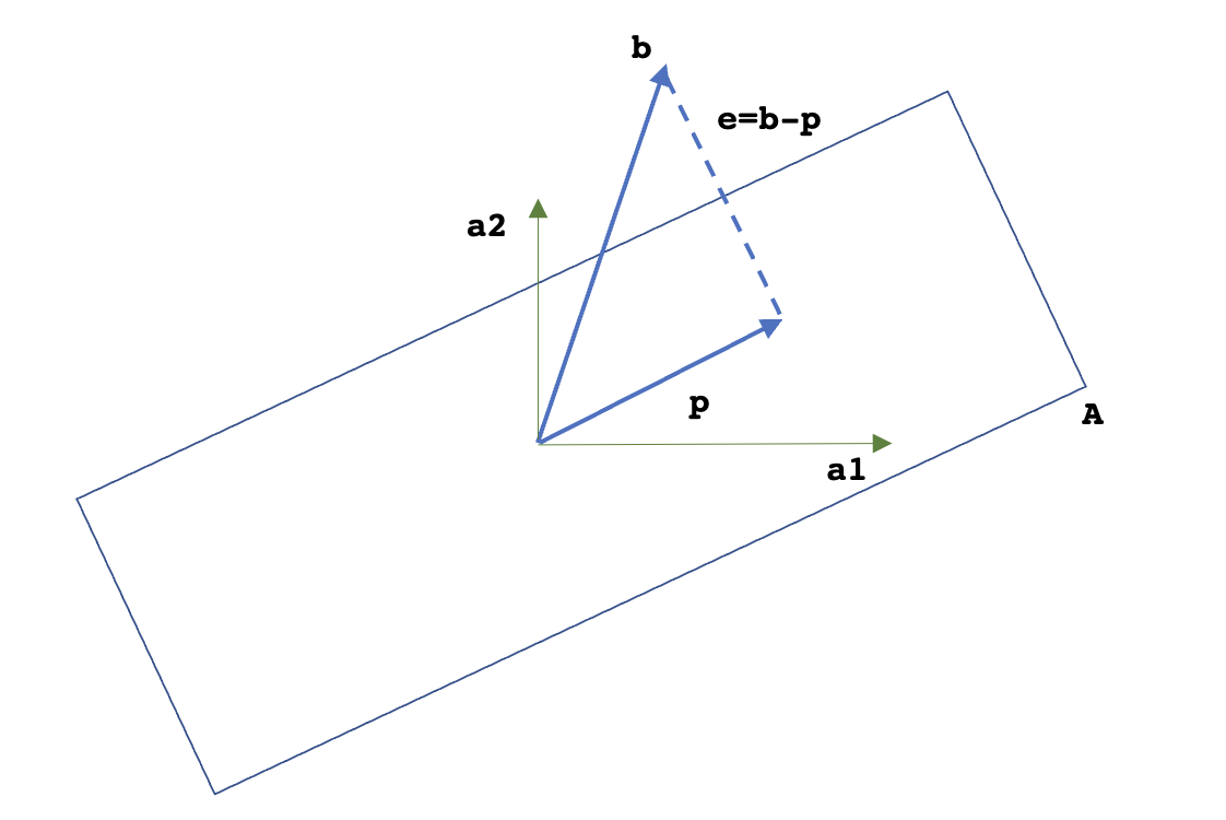
The geometrical representation of projection of $b$ onto the columnn space of $A$ is shown below. Here, projection $p$ is in the column space $C(A)$ of $A$ and is given as $p = Pb$, where $P$ is the projection matrix. The error $e$ can also be viewed as the projection of $b$ onto the null space of $A^T$, $N(A^T)$. The projection matrix for $e$ can be given as $P^{’} = I-P$ and $e = P^{’}b = (I-P)b$.

13.2 Least Squares
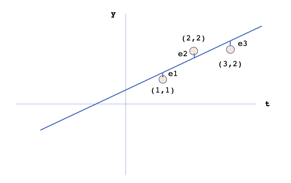
The idea behind least squares is to fit a line across multiple points. If the points are collinear, we will get a line fitting exactly across all the points. Otherwise, we won’t be able to find a line which goes through all the points. In this case, we can get a best fitting line as the one which has the minimum combined distance (called as error) from all the lines. Below figure shows an example. Individual points are $b_1,b_2,b_3$ with their projections and respective errors as: $p_1,p_2,p_3$ and $e_1,e_2,e_3$.

Let the equation of the best fitted line be $y=C+Dt$. For individual points, we get the equations as: $C+D=1;C+2D=2;C+3D=2$. In the matrix form, these equations can be reprsented as $(Ax=b)$:
$$\begin{align} \begin{bmatrix} 1 & 1 \\ 1 & 2 \\ 1 & 3 \end{bmatrix} \begin{bmatrix} C \\ D \end{bmatrix}= \begin{bmatrix} 1 \\ 2 \\ 2 \end{bmatrix}= b \end{align}$$
To get the best fitted line, we have to minimize the combined errors for all the points. These errors are $e_1, e_2, e_3$ in the figure. This error vector can be represnted as $Ax-b$. Instead of minimizing the sum of these error vectors, we can minimize their sum of squares or norm squared, which is represented as $\lVert e \rVert^2 = \lVert Ax-b \rVert^2$. So, the best fitted line can be derived by solving $Ax^{’}=b$ where $x^{’}$ is the best fitted line with parameters $x^{’} = \begin{bmatrix} C^{’} \\ D^{’} \end{bmatrix}$.
$$\begin{align} Ax^{’} = b \implies A^TAx^{’} = A^Tb \end{align}$$
$$\begin{align} A^TA = \begin{bmatrix} 1 & 1 & 1 \\ 1 & 2 & 3 \end{bmatrix} \begin{bmatrix} 1 & 1 \\ 1 & 2 \\ 1 & 3 \end{bmatrix}= \begin{bmatrix} 3 & 6 \\ 6 & 14 \end{bmatrix} \end{align}$$
$$\begin{align} A^Tb = \begin{bmatrix} 1 & 1 & 1 \\ 1 & 2 & 3 \end{bmatrix} \begin{bmatrix} 1 \\ 2 \\ 2 \end{bmatrix}= \begin{bmatrix} 5 \\ 11 \end{bmatrix} \end{align}$$
Hence, the equation get reduced as follows. Same equations can be drived by taking the partial derivatives of $\lVert e \rVert^2 = \lVert Ax-b \rVert^2 = e_1^2 + e_2^2 + e_3^2 = (C+D-1)^2 + (C+2D-2)^2 + (C+3D-2)^2$ wrt $C,D$.
$$\begin{align} \begin{bmatrix} 3 & 6 \\ 6 & 14 \end{bmatrix} \begin{bmatrix} C^{’} \\ D^{’} \end{bmatrix}= \begin{bmatrix} 5 \\ 11 \end{bmatrix} \end{align}$$
$$\begin{align} 3C^{’} + 6D^{’} = 5 \end{align}$$
$$\begin{align} 6C^{’} + 14D^{’} = 11 \end{align}$$
$$\begin{align} C = \frac{2}{3};D = \frac{1}{2} \end{align}$$
The best fit line is $y = \frac{2}{3} + \frac{1}{2}t$. The projection vector for the points is $p = \begin{bmatrix} \frac{7}{6} & \frac{10}{6} & \frac{13}{6} \end{bmatrix}^T$ with the error vector being $e = \begin{bmatrix} \frac{-1}{6} & \frac{2}{6} & \frac{-1}{6} \end{bmatrix}^T$. It should be noted that $b = p+e$. Another thing to note is $p^Te=0$, i.e. $p \perp e$. Lastly, $e$ is $\perp$ to all the vectors in the column space $C(A)$ of $A$.
One of the most importnat thing to be observed is: If $A$ has independent columns, the matrix $A^TA$ is invertible.
Proof: Suppose $A^TAx=0$. Then we have to prove that $x=0$, as if a matrix is invertible, it’s null space just have $0$ vector.
$$\begin{align} A^TAx=0 \implies x^TA^TAx=0 \implies (Ax)^T(Ax) = 0 \end{align}$$
For any vector, $y^Ty$ represents it’s length. If the length of any vector is $0$, the vector should be $0$, i.e. $Ax=0$. Finally if $A$ has independent columns and $Ax=0$, this means $x=0$.