Orthonormal Vectors, Orthogonal Matrices and Gram-Schmidt Method

14.1 Orthonormal Vectors & Orthogonal Matrices

A set of Orthonormal Vectors can be defined as:

\[\begin{align} q_i^Tq_j = \begin{cases} 0 ,& \text{if } i \neq j \\ 1 ,& \text{if } i=j \end{cases} \end{align}\]

When these set of \(n\) orthonormal vectors are put into a matrix \(Q\) such that \(Q = \begin{bmatrix} q_1 & q_2 & ... & q_n \end{bmatrix}\), then we get \(Q^TQ = I\). It should be noted that \(Q\) doesn’t have to be a square matrix. When \(Q\) is a square matrix, we can call it Orthogonal. If \(Q\) is a square matrix, \(Q^TQ=I\) gives us \(Q^T=Q^{-1}\). Hence, a square matrix whose columns are \(\perp\) to each other and are of unit length is called as orthogonal matrix. One of the example of orthogonal matrix is given below.

\[\begin{align} Q = \frac{1}{2}\begin{bmatrix} 1 & 1 & 1 & 1 \\ 1 & -1 & 1 & -1 \\ 1 & 1 & -1 & -1 \\ 1 & -1 & -1 & 1 \end{bmatrix} \end{align}\]

A rectangular matrix with orthonormal columns is shown below.

\[\begin{align} Q = \frac{1}{3}\begin{bmatrix} 1 & -2 & 2 \\ 2 & -1 & -2 \\ 2 & 2 & 1 \end{bmatrix} \end{align}\]

One of the most important property of a rectangular matrix with orthonormal columns is the ease in the computation of projection matrix \(P\). Projection matrix for any matrix \(Q\) is given as \(P=Q(Q^TQ)^{-1}Q^T\). As \(Q\) has orthonormal columns, \(Q^TQ = I\) and hence \(P=Q(Q^TQ)^{-1}Q^T = QIQ^T = QQ^T\). For an orthogonal matrix \(Q\) (square matrix with orthonormal columns), the projection matrix \(P=I\).

Now for the solution of the equation \(Ax=b\). If \(A=Q\), the equation reduces to \(Qx=b \implies Q^TQx=Q^Tb \implies x=Q^Tb\). This makes solving the equation less compue intensive as inverse of the matrix is not involved. Each individual components of \(x\) can be given as \(x_i = q_i^Tb\). Or we can say that the projection on the \(i^{th}\) basis vector is just \(q_i^Tb\).

14.2 Gram-Schmidt Method

The main goal of Gram-Schmidt Method is to convert any set of vectors into orthonormal vectors. Let \(a,b\) be two vectors. We have to convert them into orthonormal set of vectors. The conversion steps are as follows, where \(A,B\) are orthogonal vectors obtained from \(a,b\) and \(q_A,q_B\) are the final orthonormal vectors:

\[\begin{align} a,b \rightarrow A,B \rightarrow q_A = \frac{A}{\lVert A \rVert}, q_B = \frac{B}{\lVert B \rVert} \end{align}\]

We can take \(A=a\). If we revisit the way we take projection of \(b\) onto \(a\), the error \(e\) is \(\perp\) to \(a\) and hence can be taken as \(B\). i.e. \(B = e = b - \frac{A^Tb}{A^TA}A\). To confirm whether \(A \perp B\), we should have \(A^TB=0\). \(A^TB = A^T(b - \frac{A^Tb}{A^TA}A) = 0\).

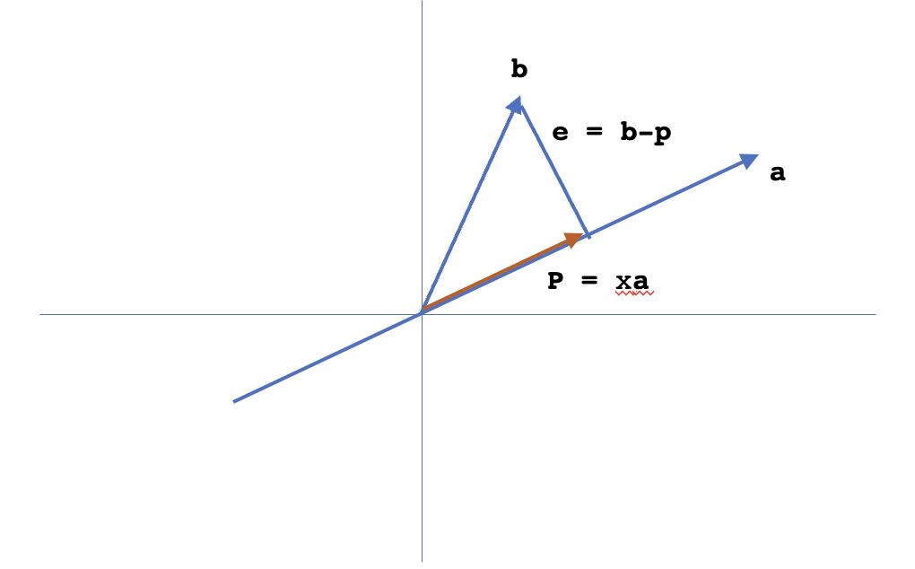
Similarly, for a set of three vectors \(a,b,c\) the transformation steps are:

\[\begin{align} a,b,c \rightarrow A,B,C \rightarrow q_A = \frac{A}{\lVert A \rVert}, q_B = \frac{B}{\lVert B \rVert}, q_C = \frac{C}{\lVert C \rVert} \end{align}\]

We can compute \(A,B\) and hence \(q_A,q_B\) the same way as we did for a two vector case. To get \(C\), we have to remove the projections of \(c\) along the direction of \(A\) and \(B\) from it. Hence, \(C = c - \frac{A^Tc}{A^TA}A - \frac{B^Tc}{B^TB}B\).

Example:

\[\begin{align} a = \begin{bmatrix} 1 \\ 1 \\ 1 \end{bmatrix}, b = \begin{bmatrix} 1 \\ 0 \\ 2 \end{bmatrix} \implies A = \begin{bmatrix} 1 \\ 1 \\ 1 \end{bmatrix}, B = \begin{bmatrix} 1 \\ 1 \\ 1 \end{bmatrix} - \frac{3}{3}\begin{bmatrix} 1 \\ 0 \\ 2 \end{bmatrix} = \begin{bmatrix} 0 \\ -1 \\ 1 \end{bmatrix} \end{align}\]\[\begin{align} q_A = \frac{1}{\sqrt{3}}\begin{bmatrix} 1 \\ 1 \\ 1 \end{bmatrix}, B = \frac{1}{\sqrt{2}}\begin{bmatrix} 0 \\ -1 \\ 1 \end{bmatrix} \end{align}\]

Finally, a matrix \(A\) whose columns are \(a,b\) and is denoted as \(A = \begin{bmatrix} a & b \end{bmatrix}\) can be decomposed as \(A=QR\) where \(Q = \begin{bmatrix} q_A & q_B \end{bmatrix}\) and \(R\) is upper triangular. \(R\) is upper triangular beacuse later columns of \(Q\) are all perpendicular to the former ones.