ISLR Chapter 10: Unsupervised Learning (Part 6: Exercises

Applied

Q7. In the chapter, we mentioned the use of correlation-based distance and Euclidean distance as dissimilarity measures for hierarchical clustering. It turns out that these two measures are almost equivalent: if each observation has been centered to have mean zero and standard deviation one, and if we let $r_{ij}$ denote the correlation between the ith and jth observations, then the quantity $1−r _{ij}$ is proportional to the squared Euclidean distance between the ith and jth observations. On the USArrests data, show that this proportionality holds.

Hint: The Euclidean distance can be calculated using the dist() function, and correlations can be calculated using the cor() function.

import pandas as pd
from sklearn.preprocessing import scale
from scipy.spatial.distance import cdist

df = pd.read_csv("data/USArrests.csv")
df.rename(columns={'Unnamed: 0': 'State'}, inplace=True)
df[['Murder', 'Assault', 'UrbanPop', 'Rape']] = scale(df[['Murder', 'Assault', 'UrbanPop', 'Rape']], axis=1)
d_euclidean = cdist(df[['Murder', 'Assault', 'UrbanPop', 'Rape']], df[['Murder', 'Assault', 'UrbanPop', 'Rape']],
          metric='euclidean')
d_correlation = cdist(df[['Murder', 'Assault', 'UrbanPop', 'Rape']], df[['Murder', 'Assault', 'UrbanPop', 'Rape']],
          metric='correlation')

df_relation = pd.DataFrame(d_euclidean**2/(1-d_correlation))
df_relation.describe()

	0	1	2	3	4	5	6	7	8	9	...	40	41	42	43	44	45	46	47	48	49
count	50.000000	50.000000	50.000000	50.000000	50.000000	50.000000	50.000000	50.000000	50.000000	50.000000	...	50.000000	50.000000	50.000000	50.000000	50.000000	50.000000	50.000000	50.000000	50.000000	50.000000
mean	0.917196	1.377766	0.768684	0.835502	0.633609	0.551528	0.636466	0.638445	0.929853	0.848389	...	0.387890	0.730992	0.490706	0.547206	0.543436	0.475501	0.400632	0.404453	3.159859	0.509535
std	2.491905	3.625065	2.114578	2.286917	1.747983	1.476750	0.579707	1.779954	2.525718	2.318681	...	0.806068	2.020526	1.366438	0.562794	0.564614	1.318453	0.867514	0.971656	2.161903	1.421946
min	0.000000	0.000000	0.000000	0.000000	0.000000	0.000000	0.000000	0.000000	0.000000	0.000000	...	0.000000	0.000000	0.000000	0.000000	0.000000	0.000000	0.000000	0.000000	0.000000	0.000000
25%	0.032012	0.089498	0.016312	0.028225	0.031815	0.052559	0.176210	0.029639	0.034926	0.032570	...	0.037003	0.014472	0.035702	0.136008	0.129466	0.032512	0.062962	0.052856	1.396576	0.040784
50%	0.194972	0.371256	0.121050	0.153813	0.123040	0.114278	0.501816	0.107965	0.195236	0.163924	...	0.166428	0.110865	0.102117	0.406559	0.416032	0.105314	0.154284	0.159624	2.840412	0.097088
75%	0.661991	1.044089	0.525318	0.588041	0.389477	0.295860	0.981708	0.393930	0.673405	0.599727	...	0.392379	0.488617	0.266171	0.846270	0.819825	0.265969	0.355743	0.274510	4.886207	0.267781
max	16.482235	24.396269	13.874904	15.058890	11.408640	9.635337	2.790843	11.655091	16.705192	15.286165	...	5.393157	13.240649	8.948936	3.163273	3.277025	8.635749	5.784783	6.473499	7.762162	9.310704

8 rows × 50 columns

Q8. In Section 10.2.3, a formula for calculating PVE was given in Equation 10.8. We also saw that the PVE can be obtained using the sdev output of the prcomp() function.

On the USArrests data, calculate PVE in two ways:

(a) Using the sdev output of the prcomp() function, as was done in Section 10.2.3.

(b) By applying Equation 10.8 directly. That is, use the prcomp() function to compute the principal component loadings. Then, use those loadings in Equation 10.8 to obtain the PVE.

import numpy as np
from sklearn.decomposition import PCA

df = pd.read_csv("data/USArrests.csv")
df.rename(columns={'Unnamed: 0': 'State'}, inplace=True)
df[['Murder', 'Assault', 'UrbanPop', 'Rape']] = scale(df[['Murder', 'Assault', 'UrbanPop', 'Rape']], axis=1)

pca = PCA(n_components=1)
principalComponents = pca.fit_transform(df[['Murder', 'Assault', 'UrbanPop', 'Rape']])
print("Variance Explained (from the model): " + str(pca.explained_variance_ratio_[0]))
print("Variance Explained (calculated manually): " + str(np.var(principalComponents)/df.var().sum()))

Variance Explained (from the model): 0.9453253030966985
Variance Explained (calculated manually): 0.926418797034764

Q9. Consider the USArrests data. We will now perform hierarchical clusteringon the states.

(a) Using hierarchical clustering with complete linkage and Euclidean distance, cluster the states.

from sklearn.cluster import AgglomerativeClustering
from scipy.cluster.hierarchy import dendrogram
from scipy.cluster.hierarchy import linkage

df = pd.read_csv("data/USArrests.csv")
df.rename(columns={'Unnamed: 0': 'State'}, inplace=True)
X = df[['Murder', 'Assault', 'UrbanPop', 'Rape']]

clustering = AgglomerativeClustering(linkage="complete", affinity="euclidean", compute_full_tree=True).fit(X)

Z = linkage(X, 'complete')
fig = plt.figure(figsize=(25, 10))
dn = dendrogram(Z, labels=df['State'].tolist())

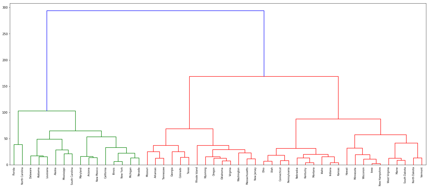
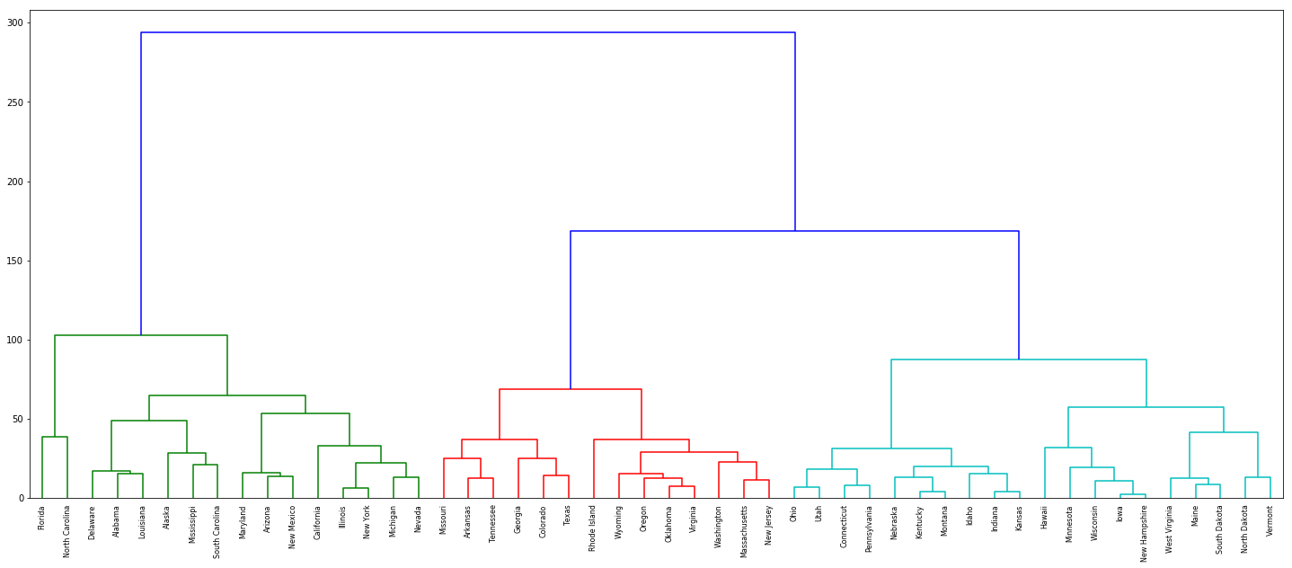
(b) Cut the dendrogram at a height that results in three distinct clusters. Which states belong to which clusters?

fig = plt.figure(figsize=(25, 10))
dn = dendrogram(Z, labels=df['State'].tolist(), color_threshold=120)

(c) Hierarchically cluster the states using complete linkage and Euclidean distance, after scaling the variables to have standard deviation one.

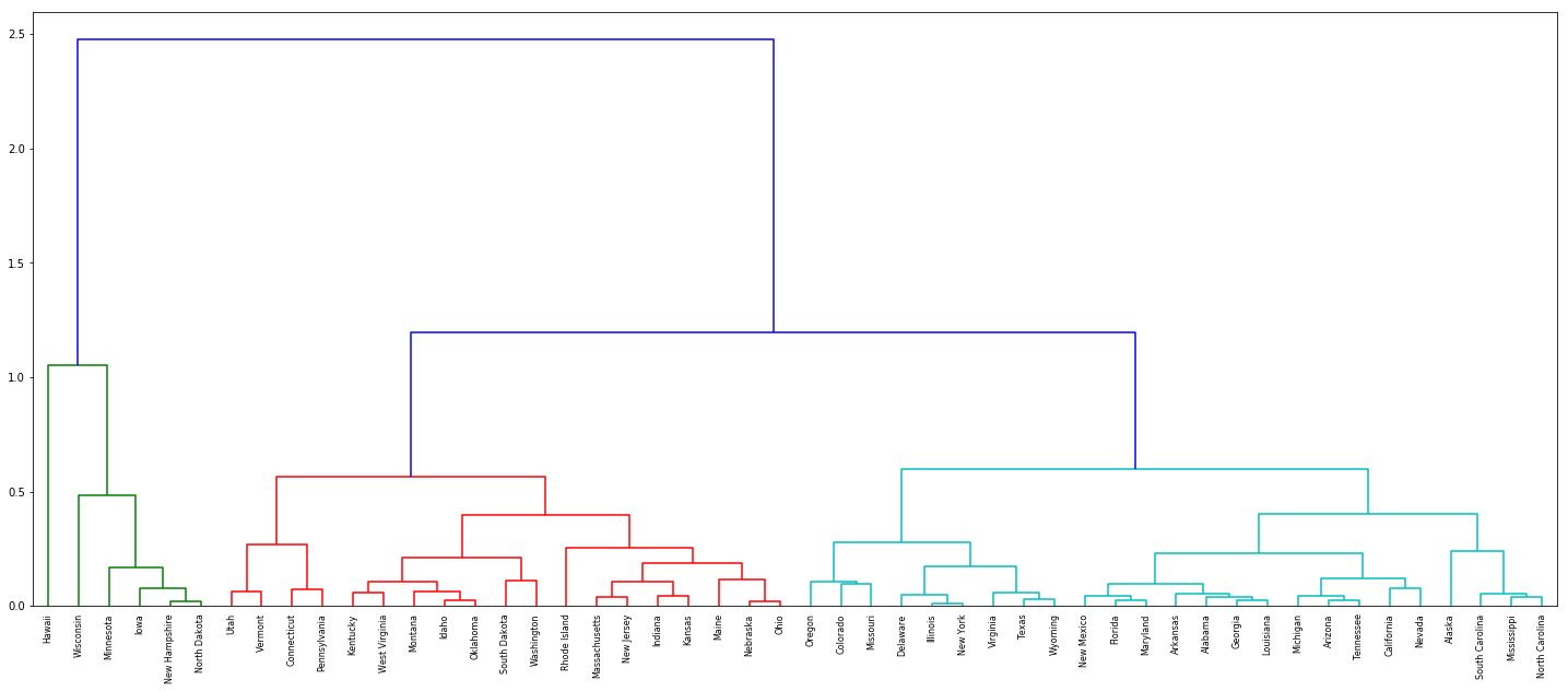
(d) What effect does scaling the variables have on the hierarchical clustering obtained? In your opinion, should the variables be scaled before the inter-observation dissimilarities are computed? Provide a justification for your answer.

Sol: The variables should be scaled as the units are different for different features.

df[['Murder', 'Assault', 'UrbanPop', 'Rape']] = scale(df[['Murder', 'Assault', 'UrbanPop', 'Rape']], axis=1)
X = df[['Murder', 'Assault', 'UrbanPop', 'Rape']]
Z = linkage(X, 'complete')
fig = plt.figure(figsize=(25, 10))
dn = dendrogram(Z, labels=df['State'].tolist())

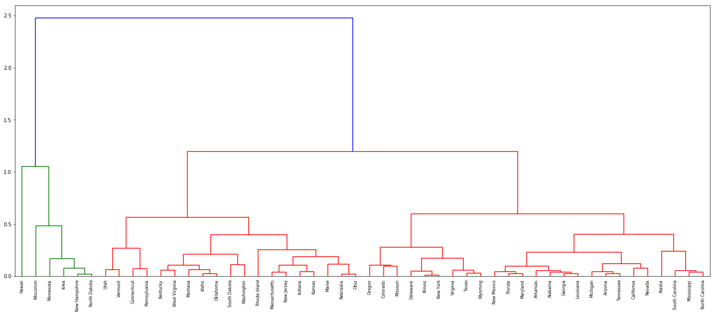
fig = plt.figure(figsize=(25, 10))
dn = dendrogram(Z, labels=df['State'].tolist(), color_threshold=1.1)

Q10. In this problem, you will generate simulated data, and then perform PCA and K-means clustering on the data.

(a) Generate a simulated data set with 20 observations in each of three classes (i.e. 60 observations total), and 50 variables.

Hint: There are a number of functions in R that you can use to generate data. One example is the rnorm() function; runif() is another option. Be sure to add a mean shift to the observations in each class so that there are three distinct classes.

np.random.seed(0)
c1 = np.append(np.random.normal(0, 0.01, (20, 50)), np.full((20, 1), 1), axis=1)
c2 = np.append(np.random.normal(0.2, 0.01, (20, 50)), np.full((20, 1), 2), axis=1)
c3 = np.append(np.random.normal(-0.2, 0.01, (20, 50)), np.full((20, 1), 3), axis=1)

df = pd.DataFrame(np.vstack((c1,c2,c3)))

(b) Perform PCA on the 60 observations and plot the first two principal component score vectors. Use a different color to indicate the observations in each of the three classes. If the three classes appear separated in this plot, then continue on to part (c). If not, then return to part (a) and modify the simulation so that there is greater separation between the three classes. Do not continue to part (c) until the three classes show at least some separation in the first two principal component score vectors.

from sklearn.decomposition import PCA

pca = PCA(n_components=2)
principalComponents = pca.fit_transform(df.iloc[:,0:50])
df_pca = pd.DataFrame(principalComponents, columns=['first', 'second'])
df_pca['labels'] = df[[50]]
df_pca.labels = df_pca.labels.astype(int)

import seaborn as sns

fig = plt.figure(figsize=(15, 8))
sns.scatterplot(x="first", y="second", hue="labels", palette={1:'green', 2:'red', 3:'blue'}, data=df_pca)
plt.grid()
plt.xlabel("First Principal Componenet")
plt.ylabel("Second Principal Componenet")
plt.show()

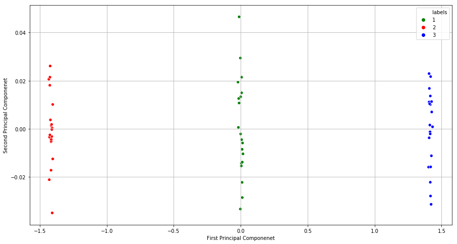
(c) Perform K-means clustering of the observations with K = 3. How well do the clusters that you obtained in K-means clustering compare to the true class labels?

Sol: The results of clustering are well in sync with the class labels.

from sklearn.cluster import KMeans

kmeans = KMeans(n_clusters=3, random_state=0).fit(df.iloc[:,0:50])
print(kmeans.labels_)

[2 2 2 2 2 2 2 2 2 2 2 2 2 2 2 2 2 2 2 2 1 1 1 1 1 1 1 1 1 1 1 1 1 1 1 1 1
 1 1 1 0 0 0 0 0 0 0 0 0 0 0 0 0 0 0 0 0 0 0 0]

(d) Perform K-means clustering with K = 2. Describe your results.

Sol: The observations belonging to first two class labels are clustered accordingly. The observations belonging to the third class label is clustered in the same group with the observations belonging to first class label.

kmeans = KMeans(n_clusters=2, random_state=0).fit(df.iloc[:,0:50])
print(kmeans.labels_)

[0 0 0 0 0 0 0 0 0 0 0 0 0 0 0 0 0 0 0 0 1 1 1 1 1 1 1 1 1 1 1 1 1 1 1 1 1
 1 1 1 0 0 0 0 0 0 0 0 0 0 0 0 0 0 0 0 0 0 0 0]

(e) Now perform K-means clustering with K = 4, and describe your results.

Sol: The observations belonging to the first two class labels are clustered accordingly. The observations belonging to the third class label is further clustered into two subgroups.

kmeans = KMeans(n_clusters=4, random_state=0).fit(df.iloc[:,0:50])
print(kmeans.labels_)

[2 2 2 2 2 2 2 2 2 2 2 2 2 2 2 2 2 2 2 2 1 1 1 1 1 1 1 1 1 1 1 1 1 1 1 1 1
 1 1 1 0 3 0 3 0 3 3 0 0 0 3 0 0 3 3 0 3 3 0 3]

(f) Now perform K-means clustering with K = 3 on the first two principal component score vectors, rather than on the raw data. That is, perform K-means clustering on the 60 × 2 matrix of which the first column is the first principal component score vector, and the second column is the second principal component score vector. Comment on the results.

Sol: The observations belonging to the last two class labels are clustered accordingly. The observations belonging to the first class label is further clustered into two subgroups.

kmeans = KMeans(n_clusters=4, random_state=0).fit(df_pca[['first', 'second']])
print(kmeans.labels_)

[3 2 3 2 2 2 2 2 3 3 2 2 2 2 3 3 3 2 3 3 1 1 1 1 1 1 1 1 1 1 1 1 1 1 1 1 1
 1 1 1 0 0 0 0 0 0 0 0 0 0 0 0 0 0 0 0 0 0 0 0]

Q11. On the book website, www.StatLearning.com, there is a gene expression data set (Ch10Ex11.csv) that consists of 40 tissue samples with measurements on 1,000 genes. The first 20 samples are from healthy patients, while the second 20 are from a diseased group.

(a) Load in the data using read.csv(). You will need to select header=F.

df = pd.read_csv("data/GeneExpression.csv", header=None)
df = df.T
df.head()

	0	1	2	3	4	5	6	7	8	9	...	990	991	992	993	994	995	996	997	998	999
0	-0.961933	-0.292526	0.258788	-1.152132	0.195783	0.030124	0.085418	1.116610	-1.218857	1.267369	...	1.325041	-0.116171	-1.470146	-0.379272	-1.465006	1.075148	-1.226125	-3.056328	1.450658	0.717977
1	0.441803	-1.139267	-0.972845	-2.213168	0.593306	-0.691014	-1.113054	1.341700	-1.277279	-0.918349	...	0.740838	-0.162392	-0.633375	-0.895521	2.034465	3.003267	-0.501702	0.449889	1.310348	0.763482
2	-0.975005	0.195837	0.588486	-0.861525	0.282992	-0.403426	-0.677969	0.103278	-0.558925	-1.253500	...	-0.435533	-0.235912	1.446660	-1.127459	0.440849	-0.123441	-0.717430	1.880362	0.383837	0.313576
3	1.417504	-1.281121	-0.800258	0.630925	0.247147	-0.729859	-0.562929	0.390963	-1.344493	-1.067114	...	-3.065529	1.597294	0.737478	-0.631248	-0.530442	-1.036740	-0.169113	-0.742841	-0.408860	-0.326473
4	0.818815	-0.251439	-1.820398	0.951772	1.978668	-0.364099	0.938194	-1.927491	1.159115	-0.240638	...	-2.378938	-0.086946	-0.122342	1.418029	1.075337	-1.270604	0.599530	2.238346	-0.471111	-0.158700

5 rows × 1000 columns

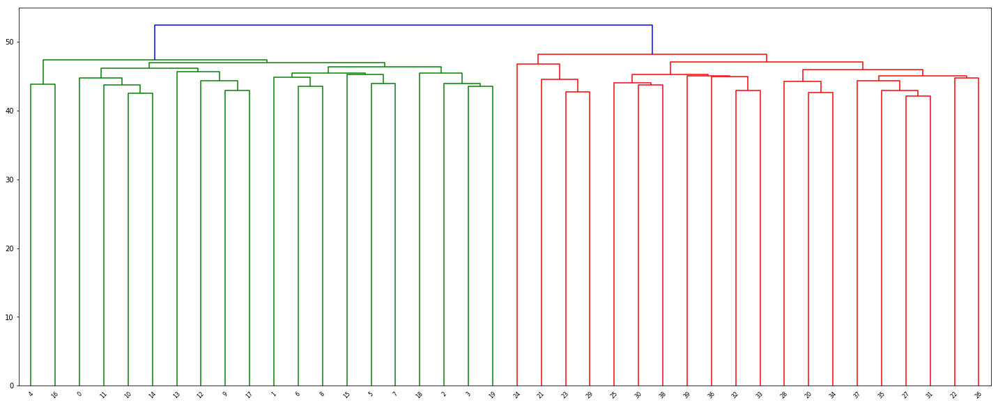
(b) Apply hierarchical clustering to the samples using correlationbased distance, and plot the dendrogram. Do the genes separate the samples into the two groups? Do your results depend on the type of linkage used?

Z = linkage(df, 'complete')
fig = plt.figure(figsize=(25, 10))
dn = dendrogram(Z, color_threshold=49)

(c) Your collaborator wants to know which genes differ the most across the two groups. Suggest a way to answer this question, and apply it here.

Sol: This can be achieved by doing PCA over the data set and reporting the genes whose loadings are maximum (as loading denotes the weight of each feature in a specified principal component) as the important genes.

ISLR Chapter 10: Unsupervised Learning (Part 6: Exercises - Applied)

Applied

CATALOG

FEATURED TAGS