10.7 Exercises
Conceptual
Q1. This problem involves the K-means clustering algorithm.
(a) Prove (10.12).
Sol: Equation 10.12 is:
$$\frac{1}{|C_k|} \sum _{i, i^{’} \in C_k} \sum _{j=1}^{p} (x _{ij} - x _{i^{’}j})^2 = 2\sum _{i \in C_k} \sum _{j=1}^{p} (x _{ij} - \bar{x} _{kj})^2$$
where $\bar{x} _{kj} = \frac{1}{|C_k|} \sum _{i \in C_k} x _{ij}$, is the mean of feature $j$ in cluster $C_k$. Expanding LHS, we get
$$\frac{1}{|C_k|} \sum _{i, i^{’} \in C_k} \sum _{j=1}^{p} (x _{ij} - x _{i^{’}j})^2 = \frac{1}{|C_k|} \sum _{i, i^{’} \in C_k} \sum _{j=1}^{p} x _{ij}^2 + \frac{1}{|C_k|} \sum _{i, i^{’} \in C_k} \sum _{j=1}^{p} x _{i^{’}j}^2 - \frac{2}{|C_k|} \sum _{i, i^{’} \in C_k} \sum _{j=1}^{p} x _{ij}x _{i^{’}j} \ = 2 \sum _{i \in C_k} \sum _{j=1}^{p} x _{ij}^2 - \frac{2}{|C_k|} \sum _{i, i^{’} \in C_k} \sum _{j=1}^{p} x _{ij}x _{i^{’}j} $$
Expanding RHS and substituting the value of $\bar{x} _{kj}$, we get
$$2\sum _{i \in C_k} \sum _{j=1}^{p} (x _{ij} - \bar{x} _{kj})^2 = 2\sum _{i \in C_k} \sum _{j=1}^{p} x _{ij}^2 - 4\sum _{i \in C_k} \sum _{j=1}^{p} x _{ij}\bar{x} _{kj}
- 2\sum _{i \in C_k} \sum _{j=1}^{p} \bar{x} _{kj}^2 = 2\sum _{i \in C_k} \sum _{j=1}^{p} x _{ij}^2 - 4|C_k| \sum _{j=1}^{p} \bar{x} _{kj}^2 + 2 |C_k| \sum _{j=1}^{p}\bar{x} _{kj}^2 = 2\sum _{i \in C_k} \sum _{j=1}^{p} x _{ij}^2 - 2|C_k| \sum _{j=1}^{p} \bar{x} _{kj}^2 = 2\sum _{i \in C_k} \sum _{j=1}^{p} x _{ij}^2 - \frac{2}{|C_k|} \sum _{i, i^{’} \in C_k} \sum _{j=1}^{p} x _{ij}x _{i^{’}j} $$
Hence, LHS and RHS are equal.
(b) On the basis of this identity, argue that the K-means clustering algorithm (Algorithm 10.1) decreases the objective (10.11) at each iteration.
Sol: As K-means clustering algorithm assigns the observations to the clusters to which they are nearest, after each iteration, the value of RHS will decrease (as this quantity is the sum of squared distance of each observation from the cluster mean). Hence, the clustering algorithm decreases the objective at each iteration.
Q2. Suppose that we have four observations, for which we compute a dissimilarity matrix, given by
$$\begin{bmatrix} & 0.3 & 0.4 & 0.7 \ 0.3 & & 0.5 & 0.8 \ 0.4 & 0.5 & & 0.45 \ 0.7 & 0.8 & 0.45 & \ \end{bmatrix}$$
For instance, the dissimilarity between the first and second observations is 0.3, and the dissimilarity between the second and fourth observations is 0.8.
(a) On the basis of this dissimilarity matrix, sketch the dendrogram that results from hierarchically clustering these four observations using complete linkage. Be sure to indicate on the plot the height at which each fusion occurs, as well as the observations corresponding to each leaf in the dendrogram.
import numpy as np

from scipy.cluster.hierarchy import dendrogram, linkage
from scipy.spatial.distance import squareform

import matplotlib.pyplot as plt

dis_mat = np.array([[0.0, 0.3, 0.4, 0.7], [0.3, 0.0, 0.5, 0.8], [0.4, 0.5, 0.0, 0.45], [0.7, 0.8, 0.45, 0.0]])
dists = squareform(dis_mat)
linkage_matrix = linkage(dists, "complete")
fig = plt.figure(figsize=(15,8))
ax = fig.add_subplot(111)
dendrogram(linkage_matrix, labels=["1", "2", "3", "4"])
plt.title("Dendrogram")
plt.show()
(b) Repeat (a), this time using single linkage clustering.
linkage_matrix = linkage(dists, "single")
fig = plt.figure(figsize=(15,8))
ax = fig.add_subplot(111)
dendrogram(linkage_matrix, labels=["1", "2", "3", "4"])
plt.title("Dendrogram")
plt.show()
(c) Suppose that we cut the dendogram obtained in (a) such that two clusters result. Which observations are in each cluster?
Sol: Observations 1 and 2 are in Cluster A and 3 and 4 in Cluster B.
(d) Suppose that we cut the dendogram obtained in (b) such that two clusters result. Which observations are in each cluster?
Sol: Observations 1, 2 and 3 are in Cluster A and 4 in Cluster B.
(e) It is mentioned in the chapter that at each fusion in the dendrogram, the position of the two clusters being fused can be swapped without changing the meaning of the dendrogram. Draw a dendrogram that is equivalent to the dendrogram in (a), for which two or more of the leaves are repositioned, but for which the meaning of the dendrogram is the same.
dis_mat = np.array([[0.0, 0.3, 0.4, 0.7], [0.3, 0.0, 0.5, 0.8], [0.4, 0.5, 0.0, 0.45], [0.7, 0.8, 0.45, 0.0]])
dists = squareform(dis_mat)
linkage_matrix = linkage(dists, "complete")
fig = plt.figure(figsize=(15,8))
ax = fig.add_subplot(111)
dendrogram(linkage_matrix, labels=["1", "4", "3", "2"])
plt.title("Dendrogram")
plt.show()
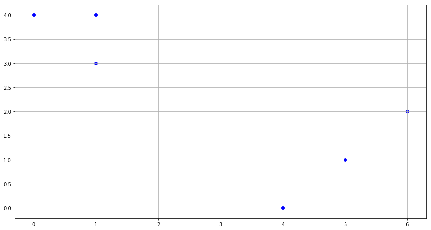
Q3. In this problem, you will perform K-means clustering manually, with K = 2, on a small example with n = 6 observations and p = 2 features. The observations are as follows.
(a) Plot the observations.
x1 = [1,1,0,5,6,4]
x2 = [4,3,4,1,2,0]
fig = plt.figure(figsize=(15,8))
plt.scatter(x1, x2, c='blue')
plt.grid()
plt.show()
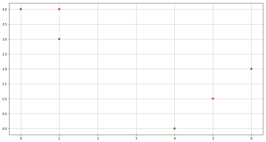
(b) Randomly assign a cluster label to each observation. You can use the sample() command in R to do this. Report the cluster labels for each observation.
np.random.seed(0)
cluster_labels = np.random.randint(2, size=6)
color= ['red' if l == 0 else 'green' for l in cluster_labels]
fig = plt.figure(figsize=(15,8))
plt.scatter(x1, x2, c=color)
plt.grid()
plt.show()
(c) Compute the centroid for each cluster.
centroid_0_x1 = 0
centroid_0_x2 = 0
centroid_1_x1 = 0
centroid_1_x2 = 0
count_0 = 0
count_1 = 0

for idx, cluster in enumerate(cluster_labels):
    if cluster == 0:
        centroid_0_x1 += x1[idx]
        centroid_0_x2 += x2[idx]
        count_0 += 1
    else:
        centroid_1_x1 += x1[idx]
        centroid_1_x2 += x2[idx]
        count_1 += 1

centroid_0_x1 = centroid_0_x1/count_0
centroid_0_x2 = centroid_0_x2/count_0
centroid_1_x1 = centroid_1_x1/count_1
centroid_1_x2 = centroid_1_x2/count_1
print("Centriod for Clutser 0 is: " + str(centroid_0_x1) + ", " + str(centroid_0_x2))
print("Centriod for Clutser 1 is: " + str(centroid_1_x1) + ", " + str(centroid_1_x2))
Centriod for Clutser 0 is: 3.0, 2.5
Centriod for Clutser 1 is: 2.75, 2.25
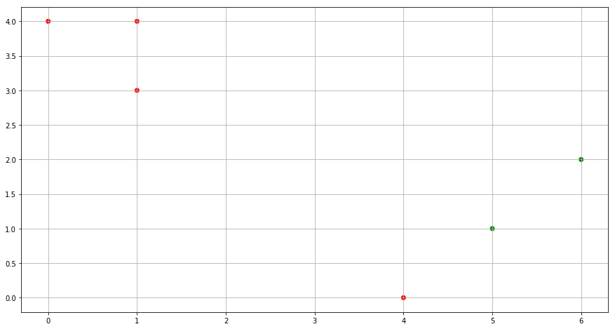
(d) Assign each observation to the centroid to which it is closest, in terms of Euclidean distance. Report the cluster labels for each observation.
for idx, cluster in enumerate(cluster_labels):
    dist_0 = (x1[idx] - centroid_0_x1)**2 + (x2[idx] - centroid_0_x2)**2
    dist_1 = (x1[idx] - centroid_1_x1)**2 + (x2[idx] - centroid_1_x2)**2
    if dist_0 > dist_1:
        cluster_labels[idx] = 0
    else:
        cluster_labels[idx] = 1

color= ['red' if l == 0 else 'green' for l in cluster_labels]
fig = plt.figure(figsize=(15,8))
plt.scatter(x1, x2, c=color)
plt.grid()
plt.show()
(e) Repeat (c) and (d) until the answers obtained stop changing.
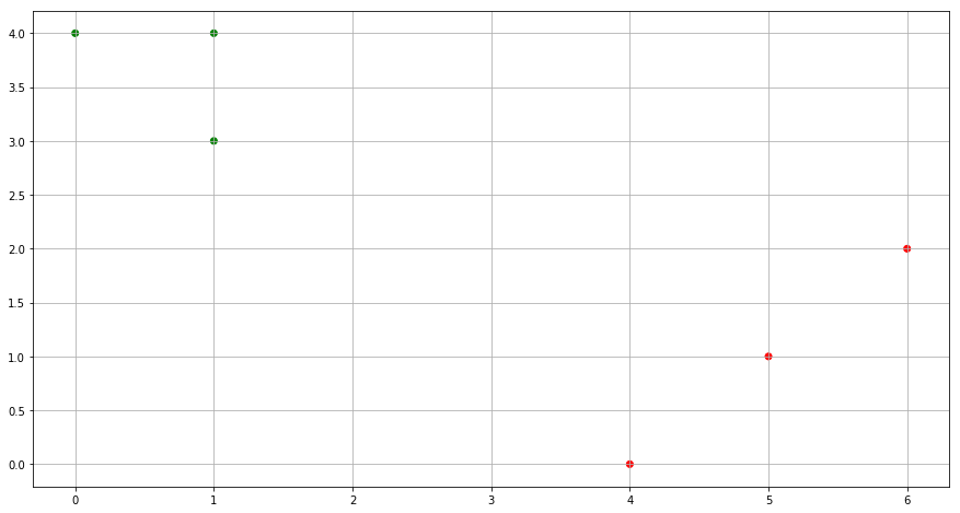
(f) In your plot from (a), color the observations according to the cluster labels obtained.
from sklearn.cluster import KMeans

M = np.column_stack((x1,x2))
kmeans = KMeans(n_clusters=2, random_state=0).fit(M)
cluster_labels = kmeans.labels_

color= ['red' if l == 0 else 'green' for l in cluster_labels]
fig = plt.figure(figsize=(15,8))
plt.scatter(x1, x2, c=color)
plt.grid()
plt.show()
Q4. Suppose that for a particular data set, we perform hierarchical clustering using single linkage and using complete linkage. We obtain two dendrograms.
(a) At a certain point on the single linkage dendrogram, the clusters {1, 2, 3} and {4, 5} fuse. On the complete linkage dendrogram, the clusters {1, 2, 3} and {4, 5} also fuse at a certain point. Which fusion will occur higher on the tree, or will they fuse at the same height, or is there not enough information to tell?
Sol: In the case of complete linkage, the fusion will occure higher on the tree as it takes into account the maximum intercluster dissimilarity as the dissimilarity of the group.
(b) At a certain point on the single linkage dendrogram, the clusters {5} and {6} fuse. On the complete linkage dendrogram, the clusters {5} and {6} also fuse at a certain point. Which fusion will occur higher on the tree, or will they fuse at the same height, or is there not enough information to tell?
Sol: With two points, the fusion will occur at the same height as the minimal (for single) and maximal (for complete) intercluster distance will be same.
Q5. In words, describe the results that you would expect if you performed K-means clustering of the eight shoppers in Figure 10.14, on the basis of their sock and computer purchases, with K = 2. Give three answers, one for each of the variable scalings displayed. Explain.
Sol: If we do the clustering on the basis of raw numbers, socks will dominate as there purchase count is higher. For the case of scaled version, the number of computer purchased should play a greater role. If we consider the clustering based on purchase amount in dollar, once again compuetr will dominate in deciding the outcome of the clustering. The graphical representation of clustering results is shown below as well.
from scipy.cluster.vq import whiten

socks = [8, 11, 7, 6, 5, 6, 7, 8]
computers = [0, 0, 0, 0, 1, 1, 1, 1]

M = np.column_stack((socks,computers))
kmeans = KMeans(n_clusters=2, random_state=0).fit(M)
cluster_labels = kmeans.labels_

color= ['red' if l == 0 else 'green' for l in cluster_labels]
fig = plt.figure(figsize=(15,8))
ax = fig.add_subplot(121)
plt.scatter(socks, computers, c=color)
ax.set_xlabel("Socks")
ax.set_ylabel("Computers")
ax.set_title("Raw Numbers")
ax.grid()

whitened = whiten(M)
kmeans = KMeans(n_clusters=2, random_state=0).fit(whitened)
cluster_labels = kmeans.labels_

color= ['red' if l == 0 else 'green' for l in cluster_labels]
ax = fig.add_subplot(122)
plt.scatter(whitened[:, 0], whitened[:, 1], c=color)
ax.set_xlabel("Socks")
ax.set_ylabel("Computers")
ax.set_title("Scaled Numbers")
ax.grid()

plt.show()