ISLR Chapter 8: Tree-Based Methods (Part 4: Exercises

Applied

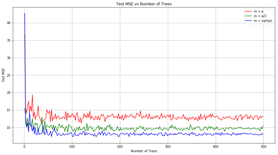
Q 7. In the lab, we applied random forests to the Boston data using mtry=6 and using ntree=25 and ntree=500. Create a plot displaying the test error resulting from random forests on this data set for a more comprehensive range of values for mtry and ntree. You can model your plot after Figure 8.10. Describe the results obtained.

import pandas as pd
from sklearn.ensemble import RandomForestRegressor
from sklearn.metrics import mean_squared_error
from sklearn.model_selection import train_test_split
from math import sqrt

boston = pd.read_csv("data/Boston.csv")
boston.dropna(inplace=True)

def random_forest_ntree(X_train, Y_train, X_test, Y_test, nTrees, max_feature):
    test_MSE = {}
    for nTree in nTrees:
        regr = RandomForestRegressor(max_features=max_feature, n_estimators=nTree)
        regr.fit(X_train, Y_train)
        p = regr.predict(X_test)
        test_MSE[nTree] = mean_squared_error(p, Y_test)
    return test_MSE

np.random.seed(5)
predictors = 13

X_train, X_test, y_train, y_test = train_test_split(boston.loc[:, boston.columns != 'medv'],
                                                    boston[['medv']], test_size=0.1)

test_MSE_p = random_forest_ntree(X_train, y_train.values.ravel(), X_test, y_test.values.ravel(), np.arange(1,300,5)
                                 , predictors)
test_MSE_pby2 = random_forest_ntree(X_train, y_train.values.ravel(), X_test, y_test.values.ravel(), np.arange(1,300,5)
                                 , int(predictors/2))
test_MSE_psqrt = random_forest_ntree(X_train, y_train.values.ravel(), X_test, y_test.values.ravel(), np.arange(1,300,5)
                                 , int(sqrt(predictors)))

fig = plt.figure(figsize=(15,8))
ax = fig.add_subplot(111)

lists = sorted(test_MSE_p.items())
x, y = zip(*lists)
plt.plot(x, y, color='r', label='m = p')

lists = sorted(test_MSE_pby2.items())
x, y = zip(*lists)
plt.plot(x, y, color='g', label='m = p/2')

lists = sorted(test_MSE_psqrt.items())
x, y = zip(*lists)
plt.plot(x, y, color='b', label='m = sqrt(p)')

ax.set_xlabel('Number of Trees')
ax.set_ylabel('Test MSE')
ax.set_title('Test MSE vs Number of Trees')

plt.grid(b=True)
plt.legend()
plt.show()

Q 8. In the lab, a classification tree was applied to the Carseats data set after converting Sales into a qualitative response variable. Now we will seek to predict Sales using regression trees and related approaches, treating the response as a quantitative variable.

(a) Split the data set into a training set and a test set.

carsets = pd.read_csv("data/Carsets.csv")
carsets['US'] = carsets['US'].map({'Yes': 1, 'No': 0})
carsets['Urban'] = carsets['Urban'].map({'Yes': 1, 'No': 0})
carsets = pd.get_dummies(carsets, prefix=['ShelveLoc'])
carsets = carsets.rename(columns={'Unnamed: 0': 'Id'})

X_train, X_test, y_train, y_test = train_test_split(carsets.drop(['Id', 'Sales'], axis=1),
                                                    carsets[['Sales']], test_size=0.1)

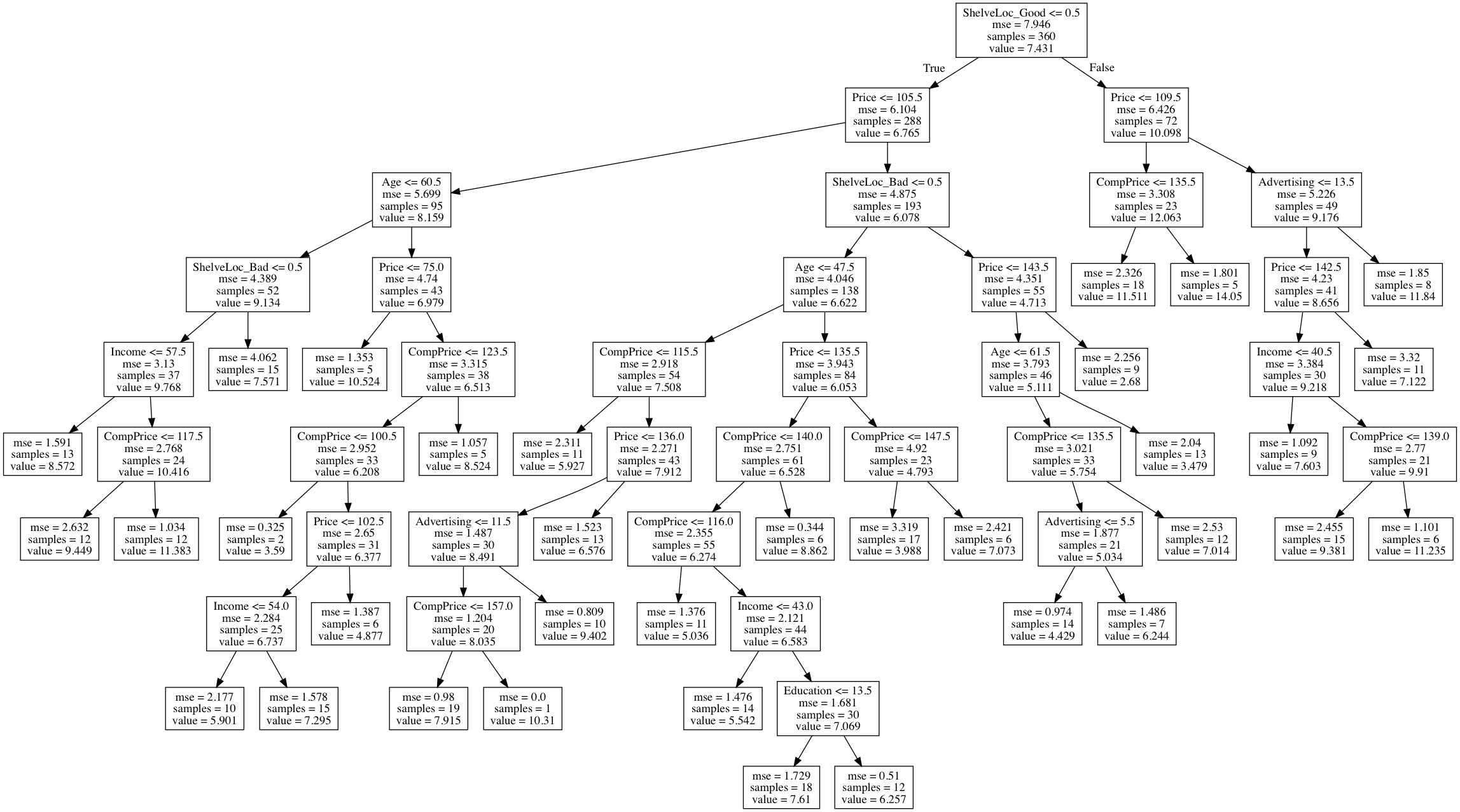
(b) Fit a regression tree to the training set. Plot the tree, and interpret the results. What test error rate do you obtain?

Sol: The stopping criteria used is: Split until there are more than 20 observations at a node. Reported test MSE is 2.6547. The regression tree is displayed below.

from sklearn.tree import DecisionTreeRegressor, export_graphviz

regressor = DecisionTreeRegressor(random_state=0, min_samples_split=20)
regressor.fit(X_train, y_train)

DecisionTreeRegressor(criterion='mse', max_depth=None, max_features=None,
           max_leaf_nodes=None, min_impurity_decrease=0.0,
           min_impurity_split=None, min_samples_leaf=1,
           min_samples_split=20, min_weight_fraction_leaf=0.0,
           presort=False, random_state=0, splitter='best')

def visualize_tree(tree, feature_names):
    """Create tree png using graphviz.

    Args
    ----
    tree -- scikit-learn DecsisionTree.
    feature_names -- list of feature names.
    """
    with open("dt.dot", 'w') as f:
        export_graphviz(tree, out_file=f,
                        feature_names=feature_names)

    command = ["dot", "-Tpng", "dt.dot", "-o", "dt.png"]
    try:
        subprocess.check_call(command)
    except:
        print("Could not run dot, ie graphviz, to "
             "produce visualization")

visualize_tree(regressor, X_train.columns.tolist())

p = regressor.predict(X_test)
print("Test MSE is: " + str(mean_squared_error(p, y_test)))

Could not run dot, ie graphviz, to produce visualization
Test MSE is: 2.6547338209551623

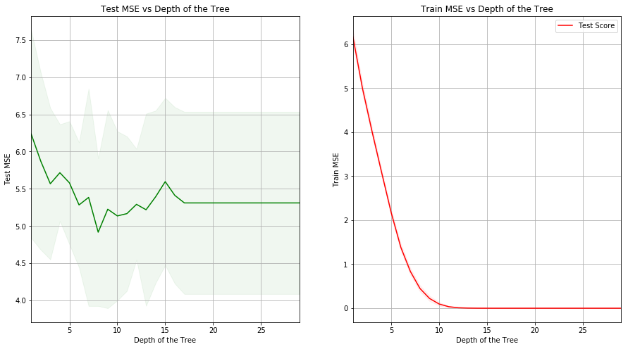
(c) Use cross-validation in order to determine the optimal level of tree complexity. Does pruning the tree improve the test error rate?

Sol: The optimal depth of tree is 8. The test MSE obtained for the mode is 3.40359.

from sklearn import tree
from sklearn.model_selection import GridSearchCV
from sklearn.metrics import mean_squared_error, make_scorer

parameters = {'max_depth':range(1,30)}
mse_scorer = make_scorer(mean_squared_error, greater_is_better=False)
clf = GridSearchCV(tree.DecisionTreeRegressor(random_state=1), parameters, n_jobs=4, cv=10,
                   scoring=mse_scorer)
clf.fit(X=X_train, y=y_train)
tree_model = clf.best_estimator_
print (clf.best_score_, clf.best_params_)

-4.917597820641044 {'max_depth': 8}

test_MSE = {}
test_MSE_std = {}
train_MSE = {}
train_MSE_std = {}
for idx, pm in enumerate(clf.cv_results_['param_max_depth'].data):
    test_MSE[pm] = abs(clf.cv_results_['mean_test_score'][idx]) # Taking absolute value as returned value of MSE is negative
    test_MSE_std[pm] = clf.cv_results_['std_test_score'][idx]
    train_MSE[pm] = abs(clf.cv_results_['mean_train_score'][idx])
    train_MSE_std[pm] = clf.cv_results_['std_train_score'][idx]

fig = plt.figure(figsize=(15,8))
ax = fig.add_subplot(121)

lists = sorted(test_MSE.items())
x, y = zip(*lists)

lists = sorted(test_MSE_std.items())
x1, y1 = zip(*lists)

plt.plot(x, y, color='g', label='Test Score')
plt.fill_between(x, np.subtract(y, y1), np.add(y, y1), alpha=0.06, color="g")
ax.set_xlabel('Depth of the Tree')
ax.set_ylabel('Test MSE')
ax.set_title('Test MSE vs Depth of the Tree')
ax.set_xlim([1, 29])
ax.grid()

ax = fig.add_subplot(122)
lists = sorted(train_MSE.items())
x, y = zip(*lists)

lists = sorted(train_MSE_std.items())
x1, y1 = zip(*lists)

plt.plot(x, y, color='r', label='Test Score')
plt.fill_between(x, np.subtract(y, y1), np.add(y, y1), alpha=0.06, color="r")
ax.set_xlabel('Depth of the Tree')
ax.set_ylabel('Train MSE')
ax.set_title('Train MSE vs Depth of the Tree')
ax.set_xlim([1, 29])
ax.grid()

plt.legend()
plt.show()

p = tree_model.predict(X_test)
print("Test MSE is: " + str(mean_squared_error(p, y_test)))

Test MSE is: 3.4035934469592464

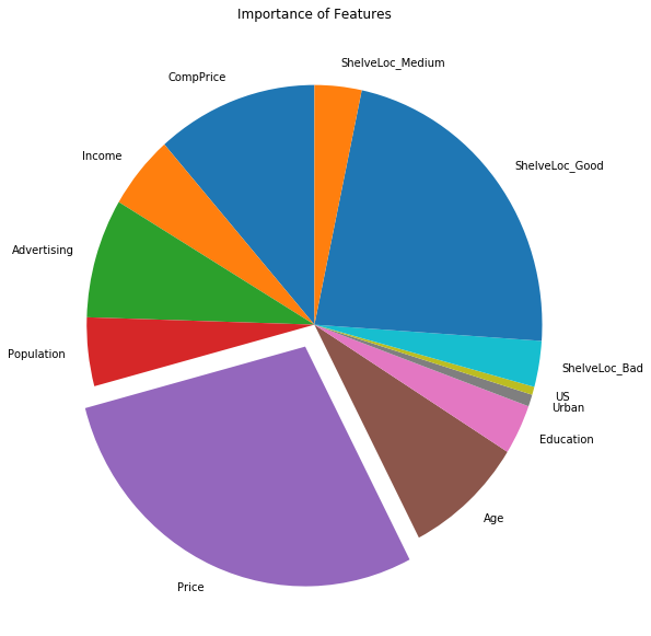
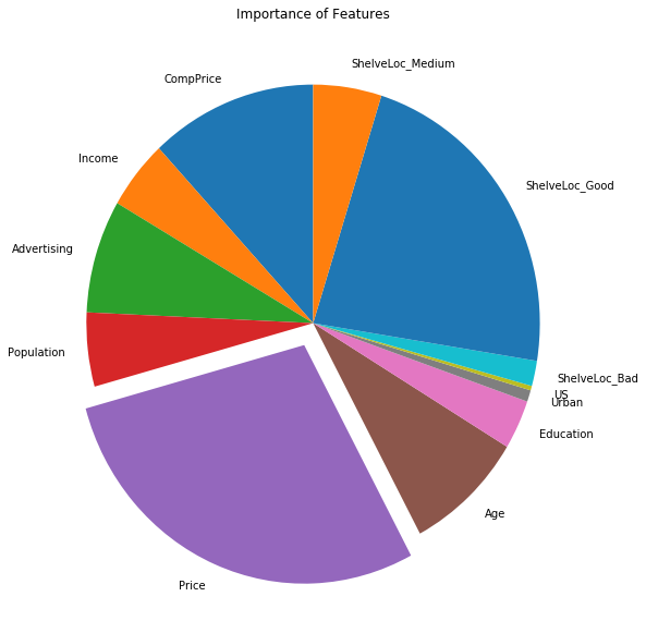
(d) Use the bagging approach in order to analyze this data. What test error rate do you obtain? Use the importance() function to determine which variables are most important.

Sol: The obtained test MSE is 2.14596. The pie-chart for importance of different features is shown as well.

from sklearn.ensemble import BaggingRegressor

bagging = BaggingRegressor(random_state=0)
bagging.fit(X=X_train, y=y_train.values.ravel())

BaggingRegressor(base_estimator=None, bootstrap=True,
         bootstrap_features=False, max_features=1.0, max_samples=1.0,
         n_estimators=10, n_jobs=1, oob_score=False, random_state=0,
         verbose=0, warm_start=False)

p = bagging.predict(X_test)
print("Test MSE is: " + str(mean_squared_error(p, y_test)))

Test MSE is: 2.145963949999999

feature_importances = np.mean([tree.feature_importances_ for tree in bagging.estimators_], axis=0)
explode = (0, 0, 0, 0, 0.1, 0, 0, 0, 0, 0, 0, 0)

fig = plt.figure(figsize=(15,8))
ax = fig.add_subplot(121)

plt.pie(feature_importances, explode=explode, labels=X_train.columns.tolist(), startangle=90)
# Equal aspect ratio ensures that pie is drawn as a circle
ax1.axis('equal')
plt.tight_layout()
plt.title("Importance of Features")
plt.show()

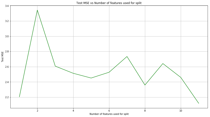
(e) Use random forests to analyze this data. What test error rate do you obtain? Use the importance() function to determine which variables are most important. Describe the effect of m, the number of variables considered at each split, on the error rate obtained.

Sol: The test MSE for random forest regressor is 2.243. Minimum test MSE is obtained when all the features are used for split.

from sklearn.ensemble import RandomForestRegressor

random_forest = RandomForestRegressor(random_state=0)
random_forest.fit(X=X_train, y=y_train.values.ravel())
p = random_forest.predict(X_test)
print("Test MSE is: " + str(mean_squared_error(p, y_test)))

Test MSE is: 2.243107725

feature_importances = np.mean([tree.feature_importances_ for tree in random_forest.estimators_], axis=0)
explode = (0, 0, 0, 0, 0.1, 0, 0, 0, 0, 0, 0, 0)

fig = plt.figure(figsize=(15,8))
ax = fig.add_subplot(121)

plt.pie(feature_importances, explode=explode, labels=X_train.columns.tolist(), startangle=90)
# Equal aspect ratio ensures that pie is drawn as a circle
ax1.axis('equal')
plt.tight_layout()
plt.title("Importance of Features")
plt.show()

def random_forest_m(X_train, Y_train, X_test, Y_test, features):
    test_MSE = {}
    for m in features:
        regr = RandomForestRegressor(random_state=0, max_features=m)
        regr.fit(X_train, Y_train)
        p = regr.predict(X_test)
        test_MSE[m] = mean_squared_error(p, Y_test)
    return test_MSE

test_MSE = random_forest_m(X_train, y_train.values.ravel(), X_test, y_test.values.ravel(),
                             np.arange(1,len(X_train.columns.tolist()),1))

fig = plt.figure(figsize=(15,8))
ax = fig.add_subplot(111)

lists = sorted(test_MSE.items())
x, y = zip(*lists)
plt.plot(x, y, color='g')

ax.set_xlabel('Number of features used for split')
ax.set_ylabel('Test MSE')
ax.set_title('Test MSE vs Number of features used for split')

plt.grid(b=True)
plt.show()

Q9. This problem involves the OJ data set which is part of the ISLR package.

(a) Create a training set containing a random sample of 800 observations, and a test set containing the remaining observations.

oj = pd.read_csv("data/OJ.csv")
oj = oj.drop(['Unnamed: 0'], axis=1)
oj['Store7'] = oj['Store7'].map({'Yes': 1, 'No': 0})
oj.head()

	Purchase	WeekofPurchase	StoreID	PriceCH	PriceMM	DiscCH	DiscMM	SpecialMM	LoyalCH	SalePriceMM	SalePriceCH	PriceDiff	Store7	PctDiscMM	PctDiscCH	ListPriceDiff	STORE
0	CH	237	1	1.75	1.99	0.00	0.0	0	0.500000	1.99	1.75	0.24	0	0.000000	0.000000	0.24	1
1	CH	239	1	1.75	1.99	0.00	0.3	1	0.600000	1.69	1.75	-0.06	0	0.150754	0.000000	0.24	1
2	CH	245	1	1.86	2.09	0.17	0.0	0	0.680000	2.09	1.69	0.40	0	0.000000	0.091398	0.23	1
3	MM	227	1	1.69	1.69	0.00	0.0	0	0.400000	1.69	1.69	0.00	0	0.000000	0.000000	0.00	1
4	CH	228	7	1.69	1.69	0.00	0.0	0	0.956535	1.69	1.69	0.00	1	0.000000	0.000000	0.00	0

X_train, X_test, y_train, y_test = train_test_split(oj.drop(['Purchase'], axis=1),
                                                    oj[['Purchase']], train_size=800)

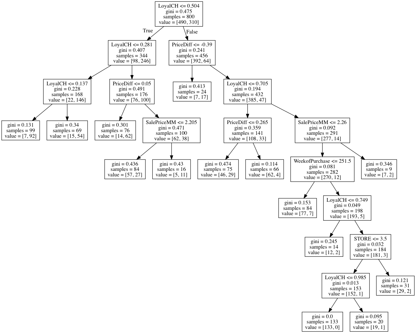
(b) Fit a tree to the training data, with Purchase as the response and the other variables except for Buy as predictors. Use the summary() function to produce summary statistics about the tree, and describe the results obtained. What is the training error rate? How many terminal nodes does the tree have?

Sol: With the stopping criteria of min_samples_split=100, training error rate is 0.1525. The most inportant features are LoyalCH and PriceDiff.

from sklearn.tree import DecisionTreeClassifier
from sklearn.metrics import accuracy_score

classifier = DecisionTreeClassifier(random_state=0, min_samples_split=100)
classifier.fit(X_train, y_train)
print("Training Error rate is: " + str(1 - accuracy_score(classifier.predict(X_train), y_train)))

Training Error rate is: 0.15249999999999997

visualize_tree(classifier, X_train.columns.tolist())

Could not run dot, ie graphviz, to produce visualization

(c) Type in the name of the tree object in order to get a detailed text output. Pick one of the terminal nodes, and interpret the information displayed.

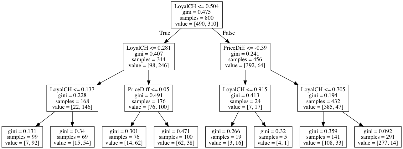
(d) Create a plot of the tree, and interpret the results.

Sol: The plot of the tree is as follows.

(e) Predict the response on the test data, and produce a confusion matrix comparing the test labels to the predicted test labels. What is the test error rate?

Sol: The test error rate is 0.21.

from sklearn.metrics import confusion_matrix
from sklearn.metrics import classification_report

p = classifier.predict(X_test)
print(confusion_matrix(p, y_test))
print(classification_report(y_test, p,))
print("Test Error rate is: " + str(1 - accuracy_score(p, y_test)))

[[139  33]
 [ 24  74]]
             precision    recall  f1-score   support

         CH       0.81      0.85      0.83       163
         MM       0.76      0.69      0.72       107

avg / total       0.79      0.79      0.79       270

Test Error rate is: 0.21111111111111114

(f) Apply the cv.tree() function to the training set in order to determine the optimal tree size.

Sol: The optimal tree depth is 3.

from sklearn import tree
from sklearn.model_selection import GridSearchCV
from sklearn.metrics import accuracy_score, make_scorer

classification_error_rate_scorer = make_scorer(accuracy_score)
parameters = {'max_depth':range(1,30)}
clf = GridSearchCV(tree.DecisionTreeClassifier(random_state=0), parameters, n_jobs=4, cv=10,
                  scoring=classification_error_rate_scorer)
clf.fit(X=X_train, y=y_train)
tree_model = clf.best_estimator_
print (clf.best_score_, clf.best_params_)

0.81625 {'max_depth': 3}

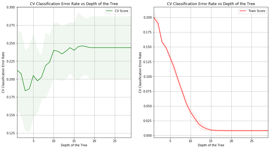
(g) Produce a plot with tree size on the x-axis and cross-validated classification error rate on the y-axis.

(h) Which tree size corresponds to the lowest cross-validated classification error rate?

Sol: Tree of depth 3 corresponds to the lowest cross-validated classification error rate.

test_MSE = {}
test_MSE_std = {}
train_MSE = {}
train_MSE_std = {}
for idx, pm in enumerate(clf.cv_results_['param_max_depth'].data):
    test_MSE[pm] = 1 - clf.cv_results_['mean_test_score'][idx]
    test_MSE_std[pm] = clf.cv_results_['std_test_score'][idx]
    train_MSE[pm] = 1 - clf.cv_results_['mean_train_score'][idx]
    train_MSE_std[pm] = clf.cv_results_['std_train_score'][idx]

fig = plt.figure(figsize=(15,8))
ax = fig.add_subplot(121)

lists = sorted(test_MSE.items())
x, y = zip(*lists)

lists = sorted(test_MSE_std.items())
x1, y1 = zip(*lists)

plt.plot(x, y, color='g', label='CV Score')
plt.fill_between(x, np.subtract(y, y1), np.add(y, y1), alpha=0.06, color="g")
ax.set_xlabel('Depth of the Tree')
ax.set_ylabel('CV Classification Error Rate')
ax.set_title('CV Classification Error Rate vs Depth of the Tree')
ax.set_xlim([1, 29])
ax.grid()
ax.legend()

ax = fig.add_subplot(122)
lists = sorted(train_MSE.items())
x, y = zip(*lists)

lists = sorted(train_MSE_std.items())
x1, y1 = zip(*lists)

plt.plot(x, y, color='r', label='Train Score')
plt.fill_between(x, np.subtract(y, y1), np.add(y, y1), alpha=0.06, color="r")
ax.set_xlabel('Depth of the Tree')
ax.set_ylabel('CV Classification Error Rate')
ax.set_title('CV Classification Error Rate vs Depth of the Tree')
ax.set_xlim([1, 29])
ax.grid()
ax.legend()

plt.show()

(i) Produce a pruned tree corresponding to the optimal tree size obtained using cross-validation. If cross-validation does not lead to selection of a pruned tree, then create a pruned tree with five terminal nodes.

Sol: The purned tree corresponding to optimal tree size is displayed below.

visualize_tree(tree_model, X_train.columns.tolist())

Could not run dot, ie graphviz, to produce visualization

(j) Compare the training error rates between the pruned and unpruned trees. Which is higher?

Sol: Training error rates for unpruned and pruned trees are 0.00875 and 0.15625 respectively. It his higher for the unpruned tree.

c = DecisionTreeClassifier(random_state=1)
c.fit(X_train, y_train)
print("Training Error rate for unpurned tree is: " + str(1 - accuracy_score(c.predict(X_train), y_train)))
print("Training Error rate for pruned tree is: " + str(1 - accuracy_score(tree_model.predict(X_train), y_train)))

Training Error rate for unpurned tree is: 0.008750000000000036
Training Error rate for pruned tree is: 0.15625

(k) Compare the test error rates between the pruned and unpruned trees. Which is higher?

Sol: Test error rates for unpruned and pruned trees are 0.2518 and 0.1926 respectively. It his higher for the pruned tree.

print("Test Error rate for unpurned tree is: " + str(1 - accuracy_score(c.predict(X_test), y_test)))
print("Test Error rate for pruned tree is: " + str(1 - accuracy_score(tree_model.predict(X_test), y_test)))

Test Error rate for unpurned tree is: 0.2518518518518519
Test Error rate for pruned tree is: 0.19259259259259254

Q10. We now use boosting to predict Salary in the Hitters data set.

(a) Remove the observations for whom the salary information is unknown, and then log-transform the salaries.

hitters = pd.read_csv("data/Hitters.csv")
hitters = hitters.rename(columns={'Unnamed: 0': 'Name'})
hitters = hitters.dropna()
hitters["Salary"] = hitters["Salary"].apply(np.log)
hitters['League'] = hitters['League'].map({'N': 1, 'A': 0})
hitters['NewLeague'] = hitters['NewLeague'].map({'N': 1, 'A': 0})
hitters['Division'] = hitters['Division'].map({'W': 1, 'E': 0})
hitters.head()

	Name	AtBat	Hits	HmRun	Runs	RBI	Walks	Years	CAtBat	CHits	...	CRuns	CRBI	CWalks	League	Division	PutOuts	Assists	Errors	Salary	NewLeague
1	-Alan Ashby	315	81	7	24	38	39	14	3449	835	...	321	414	375	1	1	632	43	10	6.163315	1
2	-Alvin Davis	479	130	18	66	72	76	3	1624	457	...	224	266	263	0	1	880	82	14	6.173786	0
3	-Andre Dawson	496	141	20	65	78	37	11	5628	1575	...	828	838	354	1	0	200	11	3	6.214608	1
4	-Andres Galarraga	321	87	10	39	42	30	2	396	101	...	48	46	33	1	0	805	40	4	4.516339	1
5	-Alfredo Griffin	594	169	4	74	51	35	11	4408	1133	...	501	336	194	0	1	282	421	25	6.620073	0

5 rows × 21 columns

(b) Create a training set consisting of the first 200 observations, and a test set consisting of the remaining observations.

train = hitters.iloc[0:200, :]
test = hitters.iloc[200:, :]

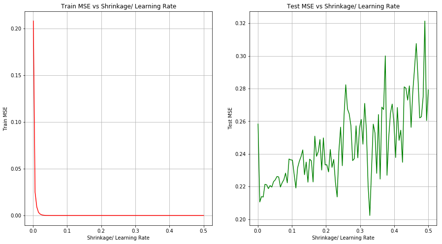
(c) Perform boosting on the training set with 1,000 trees for a range of values of the shrinkage parameter λ. Produce a plot with different shrinkage values on the x-axis and the corresponding training set MSE on the y-axis.

(d) Produce a plot with different shrinkage values on the x-axis and the corresponding test set MSE on the y-axis.

from sklearn.ensemble import GradientBoostingRegressor

def boosting_shrinkage(X_train, Y_train, X_test, Y_test, shrinkages):
    train_MSE = {}
    test_MSE = {}
    for s in shrinkages:
        clf = GradientBoostingRegressor(random_state=0, n_estimators=1000, learning_rate=s)
        clf.fit(X_train, Y_train)
        p = clf.predict(X_train)
        train_MSE[s] = mean_squared_error(p, Y_train)
        p = clf.predict(X_test)
        test_MSE[s] = mean_squared_error(p, Y_test)
    return (train_MSE, test_MSE)

X_train = train.drop(['Name', 'Salary'], axis=1)
y_train = train[['Salary']]
X_test = test.drop(['Name', 'Salary'], axis=1)
y_test = test[['Salary']]

res = boosting_shrinkage(X_train, y_train.values.ravel(), X_test, y_test.values.ravel(),
                               np.linspace(0.001, 0.5, 100))

fig = plt.figure(figsize=(15,8))

ax = fig.add_subplot(121)
lists = sorted(res[0].items())
x, y = zip(*lists)
plt.plot(x, y, color='r', label='Training Error')

ax.set_xlabel('Shrinkage/ Learning Rate')
ax.set_ylabel('Train MSE')
ax.set_title('Train MSE vs Shrinkage/ Learning Rate')
ax.grid()

ax = fig.add_subplot(122)
lists = sorted(res[1].items())
x, y = zip(*lists)
plt.plot(x, y, color='g', label='Test Error')

ax.set_xlabel('Shrinkage/ Learning Rate')
ax.set_ylabel('Test MSE')
ax.set_title('Test MSE vs Shrinkage/ Learning Rate')
ax.grid()

plt.grid(b=True)
plt.show()

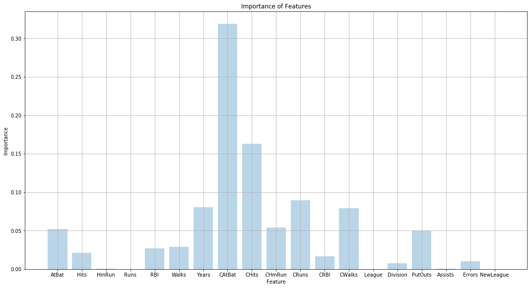
(f) Which variables appear to be the most important predictors in the boosted model?

Sol: The best boosted model is the one with learning rate of 0.1586 and uses 15 trees. The bar graph showing the importance of various features in the model is shown below.

from sklearn import ensemble
from sklearn.model_selection import GridSearchCV

parameters = {'learning_rate': np.linspace(0.001, 0.5, 20), 'n_estimators': np.arange(1, 40, 2)}
clf = GridSearchCV(ensemble.GradientBoostingRegressor(random_state=0), parameters, n_jobs=4, cv=10)
clf.fit(X=X_train, y=y_train.values.ravel())
tree_model = clf.best_estimator_
print (clf.best_score_, clf.best_params_)
p = tree_model.predict(X_test)
print("Test MSE is: " + str(mean_squared_error(p, y_test)))

0.7156560970841344 {'learning_rate': 0.15857894736842104, 'n_estimators': 15}
Test MSE is: 0.21640274598049566

feature_importances = tree_model.feature_importances_

fig = plt.figure(figsize=(15,8))
ax = fig.add_subplot(111)

plt.bar(X_train.columns.tolist(), feature_importances, alpha=0.3)

ax.set_xlabel('Feature')
ax.set_ylabel('Importance')
plt.tight_layout()
plt.title("Importance of Features")
plt.grid()
plt.show()

(g) Now apply bagging to the training set. What is the test set MSE for this approach?

Sol: Test MSE for bagging is 0.2565.

from sklearn.ensemble import BaggingRegressor

bagging = BaggingRegressor(random_state=0)
bagging.fit(X=X_train, y=y_train.values.ravel())
p = bagging.predict(X_test)
print("Test MSE is: " + str(mean_squared_error(p, y_test)))

Test MSE is: 0.25657647011895646

Q11. This question uses the Caravan data set.

(a) Create a training set consisting of the first 1,000 observations, and a test set consisting of the remaining observations.

caravan = pd.read_csv("data/Caravan.csv")
caravan = caravan.drop(['Unnamed: 0'], axis=1)
train = caravan.iloc[0:1000, :]
test = caravan.iloc[1000:, :]
print(train.shape)
print(test.shape)

(1000, 86)
(4822, 86)

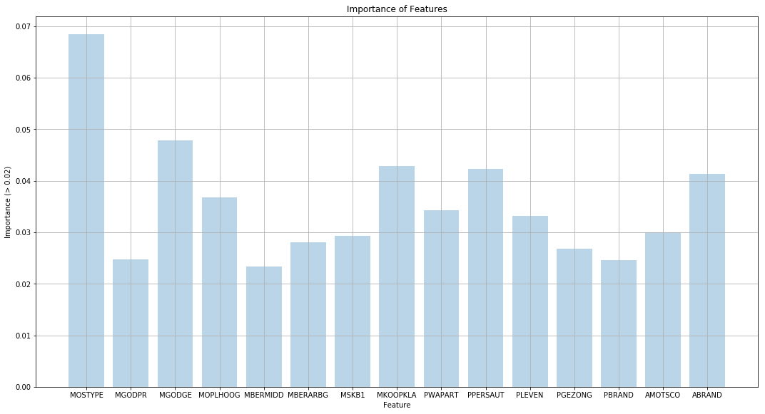
(b) Fit a boosting model to the training set with Purchase as the response and the other variables as predictors. Use 1,000 trees, and a shrinkage value of 0.01. Which predictors appear to be the most important?

from sklearn.ensemble import GradientBoostingClassifier
from sklearn.metrics import accuracy_score, make_scorer

clf = GradientBoostingClassifier(learning_rate=0.01, n_estimators=1000)

X_train = train.drop(['Purchase'], axis=1)
y_train = train[['Purchase']]
X_test = test.drop(['Purchase'], axis=1)
y_test = test[['Purchase']]

clf.fit(X=X_train, y=y_train.values.ravel())
p = clf.predict(X_test)
print("Test Error Rate is: " + str(1-accuracy_score(p, y_test)))

Test Error Rate is: 0.06656988801327246

feature_importances = clf.feature_importances_

columns, importance = zip(*((columns, importance) for columns, importance in
                   zip(X_train.columns.tolist(), clf.feature_importances_)
                   if importance > 0.02))

fig = plt.figure(figsize=(15,8))
ax = fig.add_subplot(111)

plt.bar(list(columns), list(importance), alpha=0.3)

ax.set_xlabel('Feature')
ax.set_ylabel('Importance (> 0.02)')
plt.tight_layout()
plt.title("Importance of Features")
plt.grid()
plt.show()

(c) Use the boosting model to predict the response on the test data. Predict that a person will make a purchase if the estimated probability of purchase is greater than 20 %. Form a confusion matrix. What fraction of the people predicted to make a purchase do in fact make one? How does this compare with the results obtained from applying KNN or logistic regression to this data set?

Sol: The percentage of people who are predicted to make a purchase and make one is 24.19%.

y_pred = pd.Series(p)
y_true = (y_test['Purchase'])
y_true.reset_index(drop=True, inplace=True)

pd.crosstab(y_true, y_pred, rownames=['True'], colnames=['Predicted'], margins=True)

Predicted	No	Yes	All
True
No	4486	47	4533
Yes	274	15	289
All	4760	62	4822

ISLR Chapter 8: Tree-Based Methods (Part 4: Exercises - Applied)

Applied

CATALOG

FEATURED TAGS