8.4 Exercises
Conceptual
Q2. It is mentioned in Section 8.2.3 that boosting using depth-one trees (or stumps) leads to an additive model: that is, a model of the form
$$f(X) = \sum_{j=1}^{p} f_j(X_j)$$
Explain why this is the case. You can begin with (8.12) in Algorithm 8.2.
Sol: As for depth-one trees, value of $d$ is 1. Each tree is generated by splitting the data on only one predictor and the final model is formed by adding the shrunken version of them repeatedly. Hence, in the final model:
$$\widehat{f}(x) = \sum_{b=1}^{B} \lambda \widehat{f}^b(x)$$
each additive term will depend on only one predictor leading to an additive model.
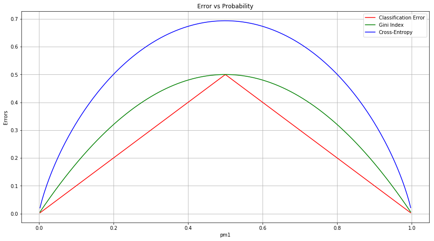
Q3. Consider the Gini index, classification error, and cross-entropy in a simple classification setting with two classes. Create a single plot that displays each of these quantities as a function of $\widehat{p}_ {m1}$. The xaxis should display $\widehat{p}_{m1}$, ranging from 0 to 1, and the y-axis should display the value of the Gini index, classification error, and entropy.
Hint: In a setting with two classes, $\widehat{p}_ {m1} = 1− \widehat{p}_ {m2}$. You could make this plot by hand, but it will be much easier to make in R.
Sol: The classification error, Gini index and cross-entropy is given as:
$$E = 1 - max_k(\widehat{p} _{mk})$$
$$G = \sum _{k=1}^{K} \widehat{p} _{mk}(1 - \widehat{p} _{mk})$$
$$D = - \sum _{k=1}^{K} \widehat{p} _{mk} log(\widehat{p} _{mk})$$
The plot showing them is as follows.
import numpy as np
import matplotlib.pyplot as plt

pm1 = np.random.uniform(0.0, 1.0, 1000)
pm2 = 1 - pm1
E = 1 - np.maximum(pm1, pm2)
G = np.add(np.multiply(pm1, pm2), np.multiply(pm1, pm2))
D = np.add(-pm1 * np.log(pm1), -pm2 * np.log(pm2))

E_dict = {}
G_dict = {}
D_dict = {}
for idx, pm in enumerate(pm1):
    E_dict[pm] = E[idx]
    G_dict[pm] = G[idx]
    D_dict[pm] = D[idx]

fig = plt.figure(figsize=(15,8))
ax = fig.add_subplot(111)

lists = sorted(E_dict.items())
x, y = zip(*lists)
plt.plot(x, y, color='r', label='Classification Error')

lists = sorted(G_dict.items())
x, y = zip(*lists)
plt.plot(x, y, color='g', label='Gini Index')

lists = sorted(D_dict.items())
x, y = zip(*lists)
plt.plot(x, y, color='b', label='Cross-Entropy')

ax.set_xlabel('pm1')
ax.set_ylabel('Errors')
ax.set_title('Error vs Probability')

plt.legend()
plt.grid()
plt.show()
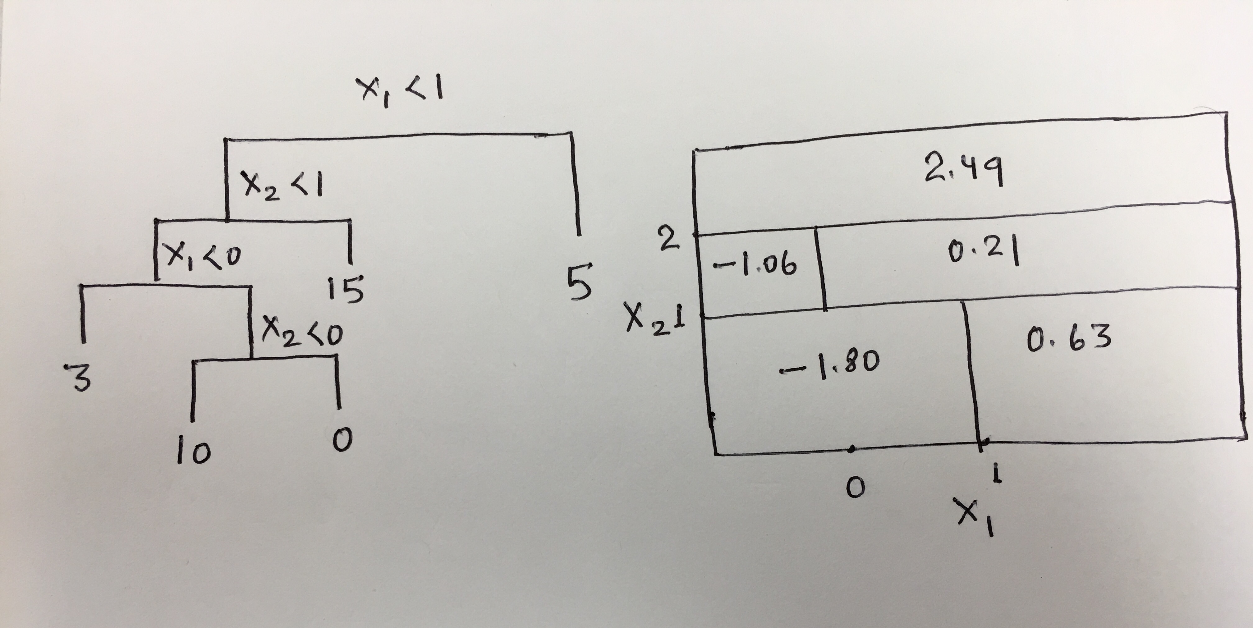
Q4. This question relates to the plots in Figure 8.12.
(a) Sketch the tree corresponding to the partition of the predictor space illustrated in the left-hand panel of Figure 8.12. The numbers inside the boxes indicate the mean of Y within each region.
(b) Create a diagram similar to the left-hand panel of Figure 8.12, using the tree illustrated in the right-hand panel of the same figure. You should divide up the predictor space into the correct regions, and indicate the mean for each region.
Sol: The diagrams are as follows:
Q5. Suppose we produce ten bootstrapped samples from a data set containing red and green classes. We then apply a classification tree to each bootstrapped sample and, for a specific value of X, produce 10 estimates of P(Class is Red|X):
0.1, 0.15, 0.2, 0.2, 0.55, 0.6, 0.6, 0.65, 0.7, and 0.75.
There are two common ways to combine these results together into a single class prediction. One is the majority vote approach discussed in this chapter. The second approach is to classify based on the average probability. In this example, what is the final classification under each of these two approaches?
Sol: For majority vote, the final classification will be the class Red, as in 6 out of 10 cases, P(Class is Red|X) > P(Class is Green|X). Here $P_ {avg}$(Class is Red|X) = 0.45 and $P_ {avg}$(Class is Green|X) = 0.55. For the classification based on average probability, the final classification is Green.