Applied
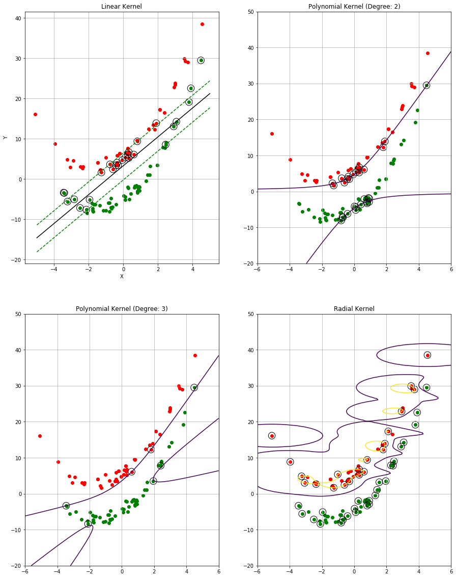
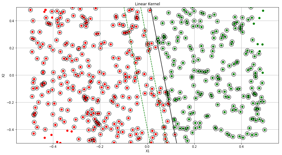
Q4. Generate a simulated two-class data set with 100 observations and two features in which there is a visible but non-linear separation between the two classes. Show that in this setting, a support vector machine with a polynomial kernel (with degree greater than 1) or a radial kernel will outperform a support vector classifier on the training data. Which technique performs best on the test data? Make plots and report training and test error rates in order to back up your assertions.
Sol: The plots with decision boundary and various error rates are shown below.
import numpy as np
from sklearn.model_selection import train_test_split
np.random.seed(0)
X = np.random.normal(0, 2, 100)
Y = X**2 + 3*X + np.random.normal(0, 1, 100)
c = list(range(0, 100))
c1 = np.random.randint(0, 100, size=50, dtype='l')
c2 = [x for x in c if x not in c1]
Y[c1] = Y[c1] + 5
Y[c2] = Y[c2] - 5
labels = np.asarray([1]*100)
labels[c2] = labels[c2] -2
M = np.column_stack((X,Y))
X_train, X_test, y_train, y_test = train_test_split(M, labels, test_size=0.1)
# fit the linear model
clf = svm.SVC(kernel='linear', C=10000)
clf.fit(X_train, y_train)
# get the separating hyperplane
w = clf.coef_[0]
a = -w[0] / w[1]
xx = np.linspace(-5, 5)
yy = a * xx - (clf.intercept_[0]) / w[1]
# plot the parallels to the separating hyperplane that pass through the
# support vectors
b = clf.support_vectors_[0]
yy_down = a * xx + (b[1] - a * b[0])
b = clf.support_vectors_[-1]
yy_up = a * xx + (b[1] - a * b[0])
fig = plt.figure(figsize=(15, 20))
ax = fig.add_subplot(221)
plt.scatter(X[c2], Y[c2], color='g')
plt.scatter(X[c1], Y[c1], color='r')
plt.scatter(clf.support_vectors_[:, 0], clf.support_vectors_[:, 1],
s=180, facecolors='none', edgecolors='black')
plt.plot(xx, yy, 'k-')
plt.plot(xx, yy_down, 'k--', color='g')
plt.plot(xx, yy_up, 'k--', color='g')
ax.set_xlabel('X')
ax.set_ylabel('Y')
ax.grid()
ax.set_title("Linear Kernel")
#fit polynomial model
clf_poly = svm.SVC(kernel='poly', degree=2, C=1000)
clf_poly.fit(X_train, y_train)
x_min = -6
x_max = 6
y_min = -20
y_max = 50
XX, YY = np.mgrid[x_min:x_max:200j, y_min:y_max:200j]
Z = clf_poly.decision_function(np.c_[XX.ravel(), YY.ravel()])
# Put the result into a color plot
Z = Z.reshape(XX.shape)
ax = fig.add_subplot(222)
plt.scatter(X[c2], Y[c2], color='g')
plt.scatter(X[c1], Y[c1], color='r')
plt.scatter(clf_poly.support_vectors_[:, 0], clf_poly.support_vectors_[:, 1],
s=180, facecolors='none', edgecolors='black')
plt.contour(XX, YY, Z, levels=[0])
ax.grid()
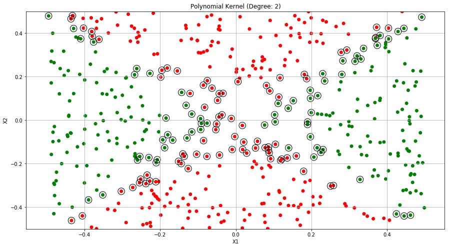
ax.set_title("Polynomial Kernel (Degree: 2)")
#fit polynomial model: degree 3
clf_poly_3 = svm.SVC(kernel='poly', degree=3, C=1000)
clf_poly_3.fit(X_train, y_train)
x_min = -6
x_max = 6
y_min = -20
y_max = 50
XX, YY = np.mgrid[x_min:x_max:200j, y_min:y_max:200j]
Z = clf_poly_3.decision_function(np.c_[XX.ravel(), YY.ravel()])
p_poly = clf_poly.predict(M)
# Put the result into a color plot
Z = Z.reshape(XX.shape)
ax = fig.add_subplot(223)
plt.scatter(X[c2], Y[c2], color='g')
plt.scatter(X[c1], Y[c1], color='r')
plt.scatter(clf_poly_3.support_vectors_[:, 0], clf_poly_3.support_vectors_[:, 1],
s=180, facecolors='none', edgecolors='black')
plt.contour(XX, YY, Z, levels=[0])
ax.grid()
ax.set_title("Polynomial Kernel (Degree: 3)")
#fit radial kernel
clf_radial = svm.SVC(kernel='rbf', C=1000)
clf_radial.fit(X_train, y_train)
Z = clf_radial.decision_function(np.c_[XX.ravel(), YY.ravel()])
# Put the result into a color plot
Z = Z.reshape(XX.shape)
ax = fig.add_subplot(224)
plt.scatter(X[c2], Y[c2], color='g')
plt.scatter(X[c1], Y[c1], color='r')
plt.scatter(clf_radial.support_vectors_[:, 0], clf_radial.support_vectors_[:, 1],
s=180, facecolors='none', edgecolors='black')
plt.contour(XX, YY, Z, levels=[0, 1])
ax.grid()
ax.set_title("Radial Kernel")
plt.show()
print("Training miss classification for linear kernel: "
      + str((len(X_train) - sum(y_train == clf.predict(X_train)))*100/len(X_train)))

print("Training miss classification for polynomial kernel (degree 2): "
      + str((len(X_train) - sum(y_train == clf_poly.predict(X_train)))*100/len(X_train)))

print("Training miss classification for polynomial kernel (degree 3): "
      + str((len(X_train) - sum(y_train == clf_poly_3.predict(X_train)))*100/len(X_train)))

print("Training miss classification for radial kernel: "
      + str((len(X_train) - sum(y_train == clf_radial.predict(X_train)))*100/len(X_train)))

print("Test miss classification for linear kernel: "
      + str((len(X_test) - sum(y_test == clf.predict(X_test)))*100/len(X_test)))

print("Test miss classification for polynomial kernel (degree 2): "
      + str((len(X_test) - sum(y_test == clf_poly.predict(X_test)))*100/len(X_test)))

print("Test miss classification for polynomial kernel (degree 3): "
      + str((len(X_test) - sum(y_test == clf_poly_3.predict(X_test)))*100/len(X_test)))

print("Test miss classification for radial kernel: "
      + str((len(X_test) - sum(y_test == clf_radial.predict(X_test)))*100/len(X_test)))
Training miss classification for linear kernel: 7.777777777777778
Training miss classification for polynomial kernel (degree 2): 16.666666666666668
Training miss classification for polynomial kernel (degree 3): 1.1111111111111112
Training miss classification for radial kernel: 0.0
Test miss classification for linear kernel: 0.0
Test miss classification for polynomial kernel (degree 2): 10.0
Test miss classification for polynomial kernel (degree 3): 0.0
Test miss classification for radial kernel: 0.0
Q5. We have seen that we can fit an SVM with a non-linear kernel in order to perform classification using a non-linear decision boundary.We will now see that we can also obtain a non-linear decision boundary by performing logistic regression using non-linear transformations of the features.
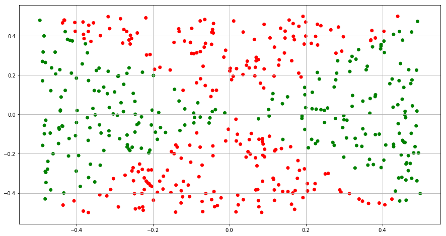
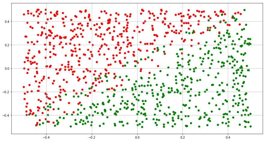
(a) Generate a data set with n = 500 and p = 2, such that the observations belong to two classes with a quadratic decision boundary between them.
(b) Plot the observations, colored according to their class labels. Your plot should display X1 on the x-axis, and X2 on the yaxis.
import matplotlib

np.random.seed(0)
X1 = np.random.uniform(0, 1, 500) - 0.5
X2 = np.random.uniform(0, 1, 500) - 0.5
Y = ((X1**2 - X2**2) > 0).astype(int)
color= ['red' if l == 0 else 'green' for l in Y]

fig = plt.figure(figsize=(15, 8))
ax = fig.add_subplot(111)

plt.scatter(X1, X2, color=color)
plt.grid()
plt.show()
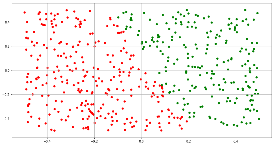
(c) Fit a logistic regression model to the data, using X1 and X2 as predictors.
(d) Apply this model to the training data in order to obtain a predicted class label for each training observation. Plot the observations, colored according to the predicted class labels. The decision boundary should be linear.
from sklearn.linear_model import LogisticRegression

X = np.column_stack((X1,X2))
clf = LogisticRegression(random_state=0, fit_intercept=True)
clf.fit(X, Y)
Y_train = clf.predict(X)

color= ['red' if l == 0 else 'green' for l in Y_train]

fig = plt.figure(figsize=(15, 8))
ax = fig.add_subplot(111)

plt.scatter(X1, X2, color=color)
plt.grid()
plt.show()
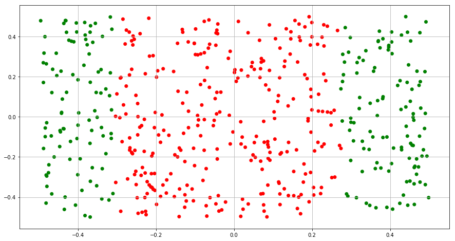
(e) Now fit a logistic regression model to the data using non-linear functions of X1 and X2 as predictors.
(f) Apply this model to the training data in order to obtain a predicted class label for each training observation. Plot the observations, colored according to the predicted class labels. The decision boundary should be obviously non-linear. If it is not, then repeat (a)-(e) until you come up with an example in which the predicted class labels are obviously non-linear.
X1_2 = X1**2
X2_2 = X1**2

X = np.column_stack((X1,X2,X1_2,X2_2))
clf = LogisticRegression(random_state=0, fit_intercept=True)
clf.fit(X, Y)
Y_train = clf.predict(X)

color= ['red' if l == 0 else 'green' for l in Y_train]

fig = plt.figure(figsize=(15, 8))
ax = fig.add_subplot(111)

plt.scatter(X1, X2, color=color)
plt.grid()
plt.show()
(g) Fit a support vector classifier to the data with X1 and X2 as predictors. Obtain a class prediction for each training observation. Plot the observations, colored according to the predicted class labels.
X = np.column_stack((X1,X2))
# fit the linear model
clf = svm.SVC(kernel='linear', C=100)
clf.fit(X, Y)
Y_train = clf.predict(X)
color= ['red' if l == 0 else 'green' for l in Y_train]

# get the separating hyperplane
w = clf.coef_[0]
a = -w[0] / w[1]
xx = np.linspace(-0.5, 0.5)
yy = a * xx - (clf.intercept_[0]) / w[1]

# plot the parallels to the separating hyperplane that pass through the
# support vectors
b = clf.support_vectors_[0]
yy_down = a * xx + (b[1] - a * b[0])
b = clf.support_vectors_[-1]
yy_up = a * xx + (b[1] - a * b[0])

fig = plt.figure(figsize=(15, 8))
ax = fig.add_subplot(111)

plt.scatter(X1, X2, color=color)
plt.scatter(clf.support_vectors_[:, 0], clf.support_vectors_[:, 1],
            s=180, facecolors='none', edgecolors='black')
plt.plot(xx, yy, 'k-')
plt.plot(xx, yy_down, 'k--', color='g')
plt.plot(xx, yy_up, 'k--', color='g')

ax.set_ylim(-0.5, 0.5)
ax.set_xlabel('X1')
ax.set_ylabel('X2')
ax.grid()
ax.set_title("Linear Kernel")
(h) Fit a SVM using a non-linear kernel to the data. Obtain a class prediction for each training observation. Plot the observations, colored according to the predicted class labels.
X = np.column_stack((X1,X2))
# fit the linear model
clf = svm.SVC(kernel='poly', degree=2, C=100)
clf.fit(X, Y)
Y_train = clf.predict(X)
color= ['red' if l == 0 else 'green' for l in Y_train]

fig = plt.figure(figsize=(15, 8))
ax = fig.add_subplot(111)

plt.scatter(X1, X2, color=color)
plt.scatter(clf.support_vectors_[:, 0], clf.support_vectors_[:, 1],
            s=180, facecolors='none', edgecolors='black')

ax.set_ylim(-0.5, 0.5)
ax.set_xlabel('X1')
ax.set_ylabel('X2')
ax.grid()
ax.set_title("Polynomial Kernel (Degree: 2)")
Q6. At the end of Section 9.6.1, it is claimed that in the case of data that is just barely linearly separable, a support vector classifier with a small value of cost that misclassifies a couple of training observations may perform better on test data than one with a huge value of cost that does not misclassify any training observations. You will now investigate this claim.
(a) Generate two-class data with p = 2 in such a way that the classes are just barely linearly separable.
np.random.seed(0)
X1 = np.random.uniform(0, 1, 1000) - 0.5
X2 = np.random.uniform(0, 1, 1000) - 0.5
X = np.column_stack((X1,X2))

temp = X1-X2
Y = [None] * len(temp)
# Assign class labels
for idx, j in enumerate(temp):
    if j > 0.1:
        Y[idx] = 1
    elif j <  -0.1:
        Y[idx] = 0
    else:
        Y[idx] = np.random.uniform(0, 1) > 0.5

color= ['red' if l == 0 else 'green' for l in Y]

fig = plt.figure(figsize=(15, 8))
ax = fig.add_subplot(111)

plt.scatter(X1, X2, color=color)
plt.grid()
plt.show()
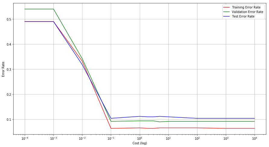
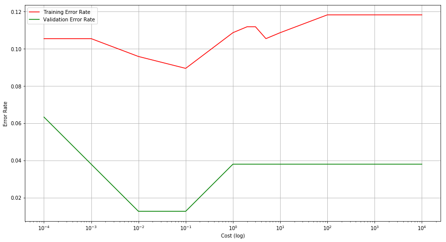
(b) Compute the cross-validation error rates for support vector classifiers with a range of cost values. How many training errors are misclassified for each value of cost considered, and how does this relate to the cross-validation errors obtained?
(c) Generate an appropriate test data set, and compute the testerrors corresponding to each of the values of cost considered. Which value of cost leads to the fewest test errors, and how does this compare to the values of cost that yield the fewest training errors and the fewest cross-validation errors?
np.random.seed(1)
X_train, X_vald, y_train, y_vald = train_test_split(X, Y, test_size=0.5)

X1_test = np.random.uniform(0, 1, 500) - 0.5
X2_test = np.random.uniform(0, 1, 500) - 0.5
X_test = np.column_stack((X1_test,X2_test))

temp_test = X1_test-X2_test
y_test = [None] * len(temp_test)
# Assign class labels
for idx, j in enumerate(temp_test):
    if j > 0.1:
        y_test[idx] = 1
    elif j <  -0.1:
        y_test[idx] = 0
    else:
        y_test[idx] = np.random.uniform(0, 1) > 0.5

cost = [0.0001, 0.001, 0.01, 0.1, 1, 2, 3, 5, 10, 100, 1000, 10000]
cross_vald_error = {}
training_error = {}
test_error= {}

for c in cost:
    clf = svm.SVC(kernel='linear', C=c)
    clf.fit(X_train, y_train)
    p = clf.predict(X_train)
    training_error[c] = (len(X_train) - sum(y_train == p))/len(X_train)
    p = clf.predict(X_vald)
    cross_vald_error[c] = (len(X_vald) - sum(y_vald == p))/len(X_vald)
    p = clf.predict(X_test)
    test_error[c] = (len(X_test) - sum(y_test == p))/len(X_test)

lists = sorted(training_error.items()) # sorted by key, return a list of tuples

x, y = zip(*lists) # unpack a list of pairs into two tuples
fig = plt.figure(figsize=(15, 8))
ax = fig.add_subplot(111)

ax.set_xscale('log')
plt.plot(x, y, color='r', label="Training Error Rate")
ax.set_xlabel("Cost (log)")
ax.set_ylabel("Error Rate")

lists = sorted(cross_vald_error.items()) # sorted by key, return a list of tuples

x, y = zip(*lists) # unpack a list of pairs into two tuples

ax.set_xscale('log')
plt.plot(x, y, color='g', label="Validation Error Rate")
ax.set_xlabel("Cost (log)")
ax.set_ylabel("Error Rate")

lists = sorted(test_error.items()) # sorted by key, return a list of tuples

x, y = zip(*lists) # unpack a list of pairs into two tuples

ax.set_xscale('log')
plt.plot(x, y, color='b', label="Test Error Rate")
ax.set_xlabel("Cost (log)")
ax.set_ylabel("Error Rate")

plt.grid()
plt.legend()
plt.show()
Q7. In this problem, you will use support vector approaches in order to predict whether a given car gets high or low gas mileage based on the Auto data set.
(a) Create a binary variable that takes on a 1 for cars with gas mileage above the median, and a 0 for cars with gas mileage below the median.
import pandas as pd

auto = pd.read_csv("data/Auto.csv")
auto.dropna(inplace=True)
auto = auto[auto['horsepower'] != '?']
auto['horsepower'] = auto['horsepower'].astype(int)
auto['mpg01'] = np.where(auto['mpg']>=auto['mpg'].median(), 1, 0)
auto.head()
| mpg | cylinders | displacement | horsepower | weight | acceleration | year | origin | name | mpg01 | |
|---|---|---|---|---|---|---|---|---|---|---|
| 0 | 18.0 | 8 | 307.0 | 130 | 3504 | 12.0 | 70 | 1 | chevrolet chevelle malibu | 0 |
| 1 | 15.0 | 8 | 350.0 | 165 | 3693 | 11.5 | 70 | 1 | buick skylark 320 | 0 |
| 2 | 18.0 | 8 | 318.0 | 150 | 3436 | 11.0 | 70 | 1 | plymouth satellite | 0 |
| 3 | 16.0 | 8 | 304.0 | 150 | 3433 | 12.0 | 70 | 1 | amc rebel sst | 0 |
| 4 | 17.0 | 8 | 302.0 | 140 | 3449 | 10.5 | 70 | 1 | ford torino | 0 |
(b) Fit a support vector classifier to the data with various values of cost, in order to predict whether a car gets high or low gas mileage. Report the cross-validation errors associated with different values of this parameter. Comment on your results.
np.random.seed(1)
X= auto[['cylinders', 'displacement', 'horsepower', 'weight', 'acceleration', 'year', 'origin']]
Y = auto[['mpg01']]
X_train, X_vald, y_train, y_vald = train_test_split(X, Y, test_size=0.2)

cost = [0.0001, 0.001, 0.01, 0.1, 1, 2, 3, 5, 10, 100, 1000, 10000]
cross_vald_error = {}
training_error = {}

for c in cost:
    clf = svm.SVC(kernel='linear', C=c)
    clf.fit(X_train, y_train.values.ravel())
    p = clf.predict(X_train)
    training_error[c] = (len(p) - sum(y_train['mpg01'] == p))/len(p)
    p = clf.predict(X_vald)
    cross_vald_error[c] = (len(p) - sum(y_vald['mpg01'] == p))/len(p)

lists = sorted(training_error.items()) # sorted by key, return a list of tuples

x, y = zip(*lists) # unpack a list of pairs into two tuples
fig = plt.figure(figsize=(15, 8))
ax = fig.add_subplot(111)

ax.set_xscale('log')
plt.plot(x, y, color='r', label="Training Error Rate")
ax.set_xlabel("Cost (log)")
ax.set_ylabel("Error Rate")

lists = sorted(cross_vald_error.items()) # sorted by key, return a list of tuples

x, y = zip(*lists) # unpack a list of pairs into two tuples

ax.set_xscale('log')
plt.plot(x, y, color='g', label="Validation Error Rate")
ax.set_xlabel("Cost (log)")
ax.set_ylabel("Error Rate")

plt.grid()
plt.legend()
plt.show()
(c) Now repeat (b), this time using SVMs with radial and polynomial basis kernels, with different values of gamma and degree and cost. Comment on your results.
from sklearn.model_selection import GridSearchCV
from sklearn.svm import SVC

parameters = {'C':[0.01, 0.1, 5, 10, 100], 'gamma':[0.01, 0.1, 5, 10, 100]}
clf = GridSearchCV(SVC(random_state=1, kernel='rbf'), parameters, n_jobs=4, cv=10)
clf.fit(X=X_train, y=y_train.values.ravel())
clf.best_estimator_
SVC(C=100, cache_size=200, class_weight=None, coef0=0.0,
  decision_function_shape='ovr', degree=3, gamma=0.01, kernel='rbf',
  max_iter=-1, probability=False, random_state=1, shrinking=True,
  tol=0.001, verbose=False)
Q8. This problem involves the OJ data set which is part of the ISLR package.
(a) Create a training set containing a random sample of 800 observations, and a test set containing the remaining observations.
np.random.seed(1)
oj = pd.read_csv("data/OJ.csv")
oj = oj.drop(['Unnamed: 0'], axis=1)
oj['Store7'] = oj['Store7'].map({'Yes': 1, 'No': 0})
X_train, X_test, y_train, y_test = train_test_split(oj.drop(['Purchase'], axis=1),
                                                    oj[['Purchase']], train_size=800)
/Users/amitrajan/Desktop/PythonVirtualEnv/Python3_VirtualEnv/lib/python3.6/site-packages/sklearn/model_selection/_split.py:2026: FutureWarning: From version 0.21, test_size will always complement train_size unless both are specified.
  FutureWarning)
(b) Fit a support vector classifier to the training data using cost=0.01, with Purchase as the response and the other variables as predictors. Use the summary() function to produce summary statistics, and describe the results obtained.
clf = svm.SVC(kernel='linear', C=0.01)
print(clf.fit(X_train, y_train.values.ravel()))
print("Number of support vectors: " +str(len(clf.support_vectors_)))
SVC(C=0.01, cache_size=200, class_weight=None, coef0=0.0,
  decision_function_shape='ovr', degree=3, gamma='auto', kernel='linear',
  max_iter=-1, probability=False, random_state=None, shrinking=True,
  tol=0.001, verbose=False)
Number of support vectors: 611
(c) What are the training and test error rates?
from sklearn.metrics import accuracy_score

print("Training Error rate is: " + str(1 - accuracy_score(clf.predict(X_train), y_train)))
print("Test Error rate is: " + str(1 - accuracy_score(clf.predict(X_test), y_test)))
Training Error rate is: 0.31000000000000005
Test Error rate is: 0.3592592592592593
(d) Use the tune() function to select an optimal cost. Consider values in the range 0.01 to 10.
parameters = {'C':[0.01, 0.05, 0.1, 0.5, 1, 2, 3, 5, 7, 8, 9, 10]}
clf = GridSearchCV(SVC(random_state=1, kernel='linear'), parameters, n_jobs=4, cv=10)
clf.fit(X=X_train, y=y_train.values.ravel())
clf.best_estimator_
SVC(C=7, cache_size=200, class_weight=None, coef0=0.0,
  decision_function_shape='ovr', degree=3, gamma='auto', kernel='linear',
  max_iter=-1, probability=False, random_state=1, shrinking=True,
  tol=0.001, verbose=False)
(e) Compute the training and test error rates using this new value for cost.
model = clf.best_estimator_
print("Training Error rate is: " + str(1 - accuracy_score(model.predict(X_train), y_train)))
print("Test Error rate is: " + str(1 - accuracy_score(model.predict(X_test), y_test)))
Training Error rate is: 0.16500000000000004
Test Error rate is: 0.16666666666666663
(f) Repeat parts (b) through (e) using a support vector machine with a radial kernel. Use the default value for gamma.
clf = GridSearchCV(SVC(random_state=1, kernel='rbf'), parameters, n_jobs=4, cv=10)
clf.fit(X=X_train, y=y_train.values.ravel())
print(clf.best_estimator_)
model = clf.best_estimator_
print("Training Error rate is: " + str(1 - accuracy_score(model.predict(X_train), y_train)))
print("Test Error rate is: " + str(1 - accuracy_score(model.predict(X_test), y_test)))
SVC(C=8, cache_size=200, class_weight=None, coef0=0.0,
  decision_function_shape='ovr', degree=3, gamma='auto', kernel='rbf',
  max_iter=-1, probability=False, random_state=1, shrinking=True,
  tol=0.001, verbose=False)
Training Error rate is: 0.15500000000000003
Test Error rate is: 0.1777777777777778