9.7 Exercises
Conceptual
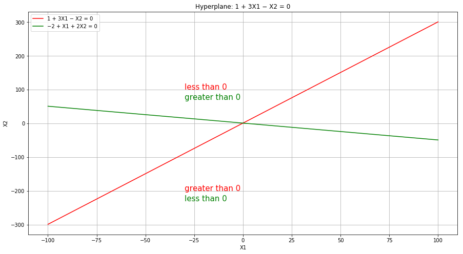
Q1. This problem involves hyperplanes in two dimensions.
(a) Sketch the hyperplane 1 + 3X1 − X2 = 0. Indicate the set of points for which 1 + 3X1 − X2 > 0, as well as the set of points for which 1 + 3X1 − X2 < 0.
(b) On the same plot, sketch the hyperplane −2 + X1 + 2X2 = 0. Indicate the set of points for which −2+ X1 +2X2 > 0, as well as the set of points for which −2+ X1 + 2X2 < 0.
import numpy as np
import matplotlib.pyplot as plt

fig = plt.figure(figsize=(15,8))
ax = fig.add_subplot(111)

x = np.linspace(-100, 100, 10000)
plt.plot(x, (1+3*x), color='r', label="1 + 3X1 − X2 = 0")
plt.text(-30, 100, "less than 0", fontdict={'color':'r', 'size':15})
plt.text(-30, -200, "greater than 0", fontdict={'color':'r', 'size':15})

plt.plot(x, (2-x)/2, color='g', label="−2 + X1 + 2X2 = 0")
plt.text(-30, 70, "greater than 0", fontdict={'color':'g', 'size':15})
plt.text(-30, -230, "less than 0", fontdict={'color':'g', 'size':15})

ax.set_xlabel('X1')
ax.set_ylabel('X2')
ax.set_title('Hyperplane: 1 + 3X1 − X2 = 0')

plt.grid()
plt.legend()
plt.show()
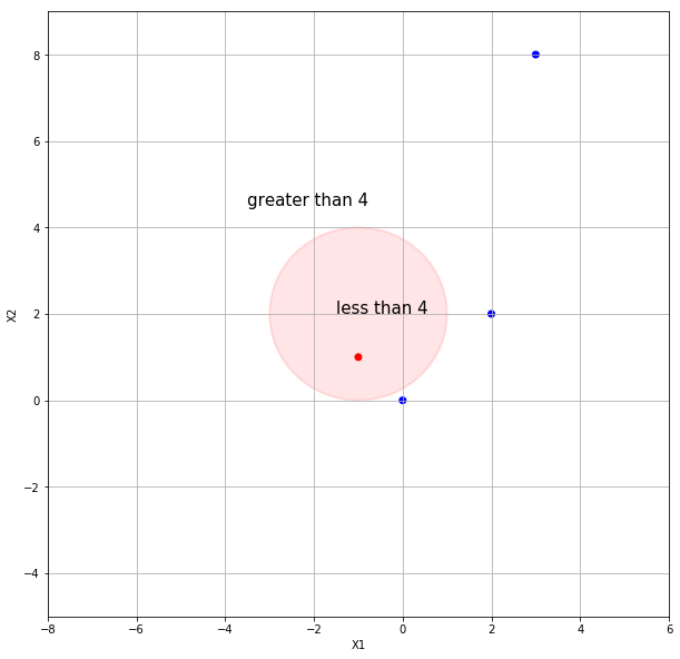
Q2. We have seen that in p = 2 dimensions, a linear decision boundary takes the form $\beta_0 + \beta_1 X_1 + \beta_2 X_2 = 0$. We now investigate a non-linear decision boundary.
(a) Sketch the curve $(1+ X_1)^2 + (2- X_2)^2 = 4$.
(b) On your sketch, indicate the set of points for which $(1+ X_1)^2 + (2- X_2)^2 > 4$, as well as the set of points for which $(1+ X_1)^2 + (2- X_2)^2 \leq 4$.
(c) Suppose that a classifier assigns an observation to the blue class if $(1+ X_1)^2 + (2- X_2)^2 > 4$, and to the red class otherwise. To what class is the observation (0, 0) classified? (−1, 1)? (2, 2)? (3, 8)?
circle = plt.Circle((-1, 2), radius=2, facecolor='r', alpha=0.1, edgecolor='r', linewidth=2.0)

fig = plt.figure(figsize=(10, 10))
ax = fig.add_subplot(111)
ax.add_artist(circle)
plt.text(-1.5, 2, "less than 4", fontdict={'color':'black', 'size':15})
plt.text(-3.5, 4.5, "greater than 4", fontdict={'color':'black', 'size':15})
plt.scatter([0, -1, 2, 3], [0, 1, 2, 8], c=['b', 'r', 'b', 'b'])

ax.set_xlim(-8, 6)
ax.set_ylim(-5, 9)
ax.set_xlabel('X1')
ax.set_ylabel('X2')

plt.grid()
plt.show()
(d) Argue that while the decision boundary in (c) is not linear in terms of $X_1$ and $X_2$, it is linear in terms of $X_1, X_2, X_1^2$ and $X_2^2$.
Sol: Expanding the above equation, we get
$$X_1^2 + X_2^2 + 2X_1 - 4X_2 = -1$$
which is linear in terms of $X_1, X_2, X_1^2$ and $X_2^2$.
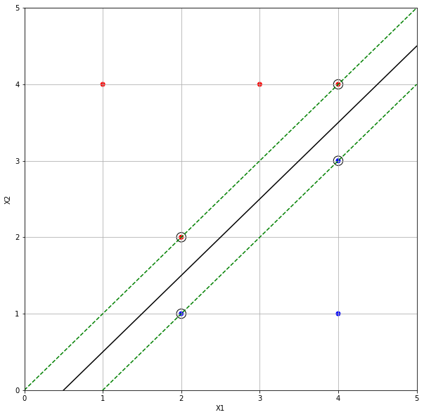
Q3. Here we explore the maximal margin classifier on a toy data set.
(a) We are given n = 7 observations in p = 2 dimensions. For each observation, there is an associated class label. Sketch the observations.
(b) Sketch the optimal separating hyperplane, and provide the equation for this hyperplane (of the form (9.1)).
Sol: The optimal separating hyperplane with margins is shown below.
(c) Describe the classification rule for the maximal margin classifier. It should be something along the lines of “Classify to Red if $\beta_0 + \beta_1 X_1 + \beta_2 X_2 > 0$, and classify to Blue otherwise.” Provide the values for $\beta_0, \beta_1, \beta_2$.
Sol: The decision boundary is given as:
$$0.99970703 -1.99941406 X_1 + 1.99941406 X_2 = 0$$
The classification rule is: Classify to Red if < 0 and Blue otherwise.
from sklearn import svm

X = [[3, 2, 4, 1, 2, 4, 4], [4, 2, 4, 4, 1, 3, 1]]
Y = ['r', 'r', 'r', 'r', 'b', 'b', 'b']

# fit the model
clf = svm.SVC(kernel='linear', C=100)
clf.fit(np.array(X).T.tolist(), Y)

# get the separating hyperplane
w = clf.coef_[0]
a = -w[0] / w[1]
xx = np.linspace(0, 5)
yy = a * xx - (clf.intercept_[0]) / w[1]

# plot the parallels to the separating hyperplane that pass through the
# support vectors
b = clf.support_vectors_[0]
yy_down = a * xx + (b[1] - a * b[0])
b = clf.support_vectors_[-1]
yy_up = a * xx + (b[1] - a * b[0])

fig = plt.figure(figsize=(10, 10))
ax = fig.add_subplot(111)

plt.scatter(clf.support_vectors_[:, 0], clf.support_vectors_[:, 1],
            s=180, facecolors='none', edgecolors='black')
plt.scatter(X[0], X[1], c=['r', 'r', 'r', 'r', 'b', 'b', 'b'])
plt.plot(xx, yy, 'k-')
plt.plot(xx, yy_down, 'k--', color='g')
plt.plot(xx, yy_up, 'k--', color='g')

ax.set_xlim(0, 5)
ax.set_ylim(0, 5)
ax.set_xlabel('X1')
ax.set_ylabel('X2')

plt.grid()
plt.show()