Applied
Q5. In Chapter 4, we used logistic regression to predict the probability of default using income and balance on the Default data set. We will now estimate the test error of this logistic regression model using the validation set approach. Do not forget to set a random seed before beginning your analysis.
import pandas as pd
import seaborn as sns
import matplotlib.pyplot as plt
import numpy as np
import statsmodels.api as sm

np.random.seed(1)
default = pd.read_excel("data/Default.xlsx")
default['student'] = default['student'].map({'Yes': 1, 'No': 0})
default['default'] = default['default'].map({'Yes': 1, 'No': 0})
(a) Fit a logistic regression model that uses income and balance to predict default.
from statsmodels.discrete.discrete_model import Logit

X = default[['income', 'balance']]
X = sm.add_constant(X, prepend=True)
y = default['default']

model = Logit(y, X)
result = model.fit()
print(result.summary())
Optimization terminated successfully.
         Current function value: 0.078948
         Iterations 10
                           Logit Regression Results
==============================================================================
Dep. Variable:                default   No. Observations:                10000
Model:                          Logit   Df Residuals:                     9997
Method:                           MLE   Df Model:                            2
Date:                Wed, 12 Sep 2018   Pseudo R-squ.:                  0.4594
Time:                        12:36:14   Log-Likelihood:                -789.48
converged:                       True   LL-Null:                       -1460.3
                                        LLR p-value:                4.541e-292
==============================================================================
                 coef    std err          z      P>|z|      [0.025      0.975]
------------------------------------------------------------------------------
const        -11.5405      0.435    -26.544      0.000     -12.393     -10.688
income      2.081e-05   4.99e-06      4.174      0.000     1.1e-05    3.06e-05
balance        0.0056      0.000     24.835      0.000       0.005       0.006
==============================================================================

Possibly complete quasi-separation: A fraction 0.14 of observations can be
perfectly predicted. This might indicate that there is complete
quasi-separation. In this case some parameters will not be identified.
(b) Using the validation set approach, estimate the test error of this model.
Sol: The estimated test error rate is 2.46%.
from sklearn.model_selection import train_test_split

train, validation = train_test_split(default, test_size=0.5)

X = train[['income', 'balance']]
X = sm.add_constant(X, prepend=True)
y = train['default']

model = Logit(y, X)
result = model.fit()
print(result.summary())

X_val = validation[['income', 'balance']]
X_val = sm.add_constant(X_val, prepend=True)
predictions = result.predict(X_val) > 0.5

print("Estimation for test error rate is: "
      +str((len(validation['default']) - np.sum(predictions == validation['default'])) / (len(validation['default']))))
Optimization terminated successfully.
         Current function value: 0.083176
         Iterations 10
                           Logit Regression Results
==============================================================================
Dep. Variable:                default   No. Observations:                 5000
Model:                          Logit   Df Residuals:                     4997
Method:                           MLE   Df Model:                            2
Date:                Wed, 12 Sep 2018   Pseudo R-squ.:                  0.4634
Time:                        12:39:27   Log-Likelihood:                -415.88
converged:                       True   LL-Null:                       -775.08
                                        LLR p-value:                1.001e-156
==============================================================================
                 coef    std err          z      P>|z|      [0.025      0.975]
------------------------------------------------------------------------------
const        -11.5308      0.604    -19.078      0.000     -12.715     -10.346
income      2.357e-05   6.78e-06      3.476      0.001    1.03e-05    3.69e-05
balance        0.0057      0.000     17.920      0.000       0.005       0.006
==============================================================================

Possibly complete quasi-separation: A fraction 0.14 of observations can be
perfectly predicted. This might indicate that there is complete
quasi-separation. In this case some parameters will not be identified.
Estimation for test error rate is: 0.0246
(c) Repeat the process in (b) three times, using three different splits of the observations into a training set and a validation set. Comment on the results obtained.
Sol: The estimated test error rate for the three cases are: 2.66%, 2.7% and 2.8%. It varies a lot along iteration.
for i in range(3):
    train, validation = train_test_split(default, test_size=0.5)

    X = train[['income', 'balance']]
    X = sm.add_constant(X, prepend=True)
    y = train['default']

    model = Logit(y, X)
    result = model.fit()

    X_val = validation[['income', 'balance']]
    X_val = sm.add_constant(X_val, prepend=True)
    predictions = result.predict(X_val) > 0.5

    print("Estimation for test error rate is: "
      +str((len(validation['default']) - np.sum(predictions == validation['default'])) / (len(validation['default']))))
Optimization terminated successfully.
         Current function value: 0.079463
         Iterations 10
Estimation for test error rate is: 0.0266
Optimization terminated successfully.
         Current function value: 0.081072
         Iterations 10
Estimation for test error rate is: 0.027
Optimization terminated successfully.
         Current function value: 0.073826
         Iterations 10
Estimation for test error rate is: 0.028
(d) Now consider a logistic regression model that predicts the probability of default using income, balance, and a dummy variable for student. Estimate the test error for this model using the validation set approach. Comment on whether or not including a dummy variable for student leads to a reduction in the test error rate.
Sol: Including student in the model does not improve the test erro rate much.
train, validation = train_test_split(default, test_size=0.5)

X = train[['income', 'balance', 'student']]
X = sm.add_constant(X, prepend=True)
y = train['default']

model = Logit(y, X)
result = model.fit()
print(result.summary())

X_val = validation[['income', 'balance', 'student']]
X_val = sm.add_constant(X_val, prepend=True)
predictions = result.predict(X_val) > 0.5

print("Estimation for test error rate is: "
      +str((len(validation['default']) - np.sum(predictions == validation['default'])) / (len(validation['default']))))
Optimization terminated successfully.
         Current function value: 0.070154
         Iterations 10
                           Logit Regression Results
==============================================================================
Dep. Variable:                default   No. Observations:                 5000
Model:                          Logit   Df Residuals:                     4996
Method:                           MLE   Df Model:                            3
Date:                Wed, 12 Sep 2018   Pseudo R-squ.:                  0.4739
Time:                        12:47:51   Log-Likelihood:                -350.77
converged:                       True   LL-Null:                       -666.74
                                        LLR p-value:                1.191e-136
==============================================================================
                 coef    std err          z      P>|z|      [0.025      0.975]
------------------------------------------------------------------------------
const        -11.3053      0.760    -14.878      0.000     -12.795      -9.816
income     -1.877e-06   1.22e-05     -0.154      0.878   -2.58e-05    2.21e-05
balance        0.0061      0.000     16.602      0.000       0.005       0.007
student       -0.9074      0.348     -2.610      0.009      -1.589      -0.226
==============================================================================

Possibly complete quasi-separation: A fraction 0.19 of observations can be
perfectly predicted. This might indicate that there is complete
quasi-separation. In this case some parameters will not be identified.
Estimation for test error rate is: 0.0306
Q6. We continue to consider the use of a logistic regression model to predict the probability of default using income and balance on the Default data set. In particular, we will now compute estimates for the standard errors of the income and balance logistic regression coefficients in two different ways: (1) using the bootstrap, and (2) using the standard formula for computing the standard errors in the glm() function. Do not forget to set a random seed before beginning your analysis.
(a) Using the summary() and glm() functions, determine the estimated standard errors for the coefficients associated with income and balance in a multiple logistic regression model that uses both predictors.
Sol: The standard errors for the coefficients are 0.435, 4.99e-06 and 0.000 respectively.
from statsmodels.discrete.discrete_model import Logit

X = default[['income', 'balance']]
X = sm.add_constant(X, prepend=True)
y = default['default']

model = Logit(y, X)
result = model.fit()
print(result.summary())
Optimization terminated successfully.
         Current function value: 0.078948
         Iterations 10
                           Logit Regression Results
==============================================================================
Dep. Variable:                default   No. Observations:                10000
Model:                          Logit   Df Residuals:                     9997
Method:                           MLE   Df Model:                            2
Date:                Wed, 12 Sep 2018   Pseudo R-squ.:                  0.4594
Time:                        13:21:36   Log-Likelihood:                -789.48
converged:                       True   LL-Null:                       -1460.3
                                        LLR p-value:                4.541e-292
==============================================================================
                 coef    std err          z      P>|z|      [0.025      0.975]
------------------------------------------------------------------------------
const        -11.5405      0.435    -26.544      0.000     -12.393     -10.688
income      2.081e-05   4.99e-06      4.174      0.000     1.1e-05    3.06e-05
balance        0.0056      0.000     24.835      0.000       0.005       0.006
==============================================================================

Possibly complete quasi-separation: A fraction 0.14 of observations can be
perfectly predicted. This might indicate that there is complete
quasi-separation. In this case some parameters will not be identified.
(b) Write a function, boot.fn(), that takes as input the Default data set as well as an index of the observations, and that outputs the coefficient estimates for income and balance in the multiple logistic regression model.
from sklearn.utils import resample

def boot(df):
    return resample(df)

train = boot(default)
X = train[['income', 'balance']]
X = sm.add_constant(X, prepend=True)
y = train['default']

model = Logit(y, X)
result = model.fit()
print(result.summary())
Optimization terminated successfully.
         Current function value: 0.076003
         Iterations 10
                           Logit Regression Results
==============================================================================
Dep. Variable:                default   No. Observations:                10000
Model:                          Logit   Df Residuals:                     9997
Method:                           MLE   Df Model:                            2
Date:                Wed, 12 Sep 2018   Pseudo R-squ.:                  0.4672
Time:                        13:34:46   Log-Likelihood:                -760.03
converged:                       True   LL-Null:                       -1426.5
                                        LLR p-value:                3.634e-290
==============================================================================
                 coef    std err          z      P>|z|      [0.025      0.975]
------------------------------------------------------------------------------
const        -11.8500      0.449    -26.380      0.000     -12.730     -10.970
income      2.468e-05   5.02e-06      4.919      0.000    1.48e-05    3.45e-05
balance        0.0057      0.000     24.615      0.000       0.005       0.006
==============================================================================

Possibly complete quasi-separation: A fraction 0.15 of observations can be
perfectly predicted. This might indicate that there is complete
quasi-separation. In this case some parameters will not be identified.
(c) Use the boot() function to estimate the standard errors of the logistic regression coefficients for income and balance.
Sol: The standard errors for the coefficients are 0.4212, 4.554e-06 and 0.00022 respectively.
B = 1000

intercept = []
income = []
balance = []

for i in range(B):
    train = boot(default)
    X = train[['income', 'balance']]
    X = sm.add_constant(X, prepend=True)
    y = train['default']

    model = Logit(y, X)
    result = model.fit(disp=False)
    intercept.append(result.params.const)
    income.append(result.params.income)
    balance.append(result.params.balance)

print("SE for intercept: " +str(np.std(intercept, ddof=1)))
print("SE for income: " +str(np.std(income, ddof=1)))
print("SE for balance: " +str(np.std(balance, ddof=1)))
SE for intercept: 0.421160671038164
SE for income: 4.5539698907803916e-06
SE for balance: 0.00022086255501253455
(d) Comment on the estimated standard errors obtained using the glm() function and using your bootstrap function.
Sol: The standard errors obtained using both of the methods are in accordance.
Q7. You will now take this approach in order to compute the LOOCV error for a simple logistic regression model on the Weekly data set.
(a) Fit a logistic regression model that predicts Direction using Lag1 and Lag2.
weekly = pd.read_csv("data/Weekly.csv")
weekly['trend'] = weekly['Direction'].map({'Down': 0, 'Up': 1})

X = weekly[['Lag1', 'Lag2']]
X = sm.add_constant(X, prepend=True)
y = weekly['trend']

model = Logit(y, X)
result = model.fit()
print(result.summary())
Optimization terminated successfully.
         Current function value: 0.683297
         Iterations 4
                           Logit Regression Results
==============================================================================
Dep. Variable:                  trend   No. Observations:                 1089
Model:                          Logit   Df Residuals:                     1086
Method:                           MLE   Df Model:                            2
Date:                Wed, 12 Sep 2018   Pseudo R-squ.:                0.005335
Time:                        14:01:38   Log-Likelihood:                -744.11
converged:                       True   LL-Null:                       -748.10
                                        LLR p-value:                   0.01848
==============================================================================
                 coef    std err          z      P>|z|      [0.025      0.975]
------------------------------------------------------------------------------
const          0.2212      0.061      3.599      0.000       0.101       0.342
Lag1          -0.0387      0.026     -1.477      0.140      -0.090       0.013
Lag2           0.0602      0.027      2.270      0.023       0.008       0.112
==============================================================================
(b) Fit a logistic regressionmodel that predicts Direction using Lag1 and Lag2 using all but the first observation.
train = weekly.iloc[1:len(weekly),:]
test = weekly.iloc[0:1, :]

X = train[['Lag1', 'Lag2']]
X = sm.add_constant(X, prepend=True)
y = train['trend']

model = Logit(y, X)
result = model.fit()
print(result.summary())
Optimization terminated successfully.
         Current function value: 0.683147
         Iterations 4
                           Logit Regression Results
==============================================================================
Dep. Variable:                  trend   No. Observations:                 1088
Model:                          Logit   Df Residuals:                     1085
Method:                           MLE   Df Model:                            2
Date:                Wed, 12 Sep 2018   Pseudo R-squ.:                0.005387
Time:                        14:41:45   Log-Likelihood:                -743.26
converged:                       True   LL-Null:                       -747.29
                                        LLR p-value:                   0.01785
==============================================================================
                 coef    std err          z      P>|z|      [0.025      0.975]
------------------------------------------------------------------------------
const          0.2232      0.061      3.630      0.000       0.103       0.344
Lag1          -0.0384      0.026     -1.466      0.143      -0.090       0.013
Lag2           0.0608      0.027      2.291      0.022       0.009       0.113
==============================================================================
(c) Use the model from (b) to predict the direction of the first observation. You can do this by predicting that the first observation will go up if P(Direction=“Up”|Lag1, Lag2) > 0.5. Was this observation correctly classified?
Sol: The observation is not correctly classified as the prediction is Up but true trend is Down.
X = test[['Lag1', 'Lag2']]
X = sm.add_constant(X, prepend=True, has_constant='add')
predictions = result.predict(X) > 0.5
print("Prediction: " + str(predictions[0]))
Prediction: True
(d) Write a for loop from i = 1 to i = n, where n is the number of observations in the data set, that performs each of the following steps:
- Fit a logistic regression model using all but the ith observation to predict Direction using Lag1 and Lag2.
- Compute the posterior probability of the market moving up for the ith observation.
- Use the posterior probability for the ith observation in order to predict whether or not the market moves up.
- Determine whether or not an error was made in predicting the direction for the ith observation. If an error was made, then indicate this as a 1, and otherwise indicate it as a 0.
n = len(weekly)

error = []
for i in range(n):
    test = weekly.iloc[[i]]
    train = weekly.drop(weekly.index[i])

    X = train[['Lag1', 'Lag2']]
    X = sm.add_constant(X, prepend=True)
    y = train['trend']

    model = Logit(y, X)
    result = model.fit(disp=False)

    X = test[['Lag1', 'Lag2']]
    X = sm.add_constant(X, prepend=True, has_constant='add')
    predictions = result.predict(X).iloc[0] > 0.5
    error.append(predictions == test['trend'].iloc[0])
(e) Take the average of the n numbers obtained in (d)iv in order to obtain the LOOCV estimate for the test error. Comment on the results.
Sol: The LOOCV estimate for the test error is 0.44995.
print("LOOCV estimate for the test error is: " + str((len(error) - sum(error)) / (len(error))))
LOOCV estimate for the test error is: 0.44995408631772266
Q8. We will now perform cross-validation on a simulated data set.
(a) Generate a simulated data set as follows:
set .seed (1) y=rnorm (100) x=rnorm (100) y=x-2* x^2+ rnorm (100)
In this data set, what is n and what is p? Write out the model used to generate the data in equation form.
Sol: In this data set, $n=100$ and $p=2$. The model used is:
$$Y = X - 2X^2 + \epsilon$$
np.random.seed(1)
x = np.random.normal(loc=0, scale=1, size=100)
y = x - 2*(x**2) + np.random.normal(loc=0, scale=1, size=100)
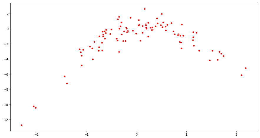
(b) Create a scatterplot of X against Y . Comment on what you find.
Sol: The scatterplot suggests a quadratic relationship.
fig = plt.figure(figsize=(15, 8))
sns.scatterplot(x=x, y=y, color='r')
(c) Set a random seed, and then compute the LOOCV errors that result from fitting the following four models using least squares:
i. Y = β0 + β1X + e
ii. Y = β0 + β1X + β2X2 + e
iii. Y = β0 + β1X + β2X2 + β3X3 + e
iv. Y = β0 + β1X + β2X2 + β3X3 + β4X4 + e
Sol: Instead models upto 7th power of X has been fitted. The model with 4 parameters has the lowest LOOCV error.
import random
from sklearn.linear_model import LinearRegression

def LOOCV(df):
    n = len(df)
    error = 0.0

    for i in range(n):
        test = df.iloc[[i]]
        train = df.drop(df.index[i])

        X_ = train.loc[:, train.columns != 'y']
        y_ = train['y']

        model = LinearRegression(fit_intercept=True)
        model.fit (X_, y_)

        X_ = test.loc[:, df.columns != 'y']
        predictions = model.predict(X_)
        error += (predictions - test.iloc[0]['y'])**2

    return (error/n)

random.seed(1)
# Model 1
df = pd.DataFrame({'x':x, 'y':y})
print("MSE for model 1: " +str(LOOCV(df)))

# Model 1
df = pd.DataFrame({'x':x, 'x2':x**2, 'y':y})
print("MSE for model 2: " +str(LOOCV(df)))

# Model 3
df = pd.DataFrame({'x':x, 'x2':x**2, 'x3':x**3, 'y':y})
print("MSE for model 3: " +str(LOOCV(df)))

# Model 4
df = pd.DataFrame({'x':x, 'x2':x**2, 'x3':x**3, 'x4':x**4, 'y':y})
print("MSE for model 4: " +str(LOOCV(df)))

# Model 5
df = pd.DataFrame({'x':x, 'x2':x**2, 'x3':x**3, 'x4':x**4, 'x5':x**5, 'y':y})
print("MSE for model 5: " +str(LOOCV(df)))

# Model 6
df = pd.DataFrame({'x':x, 'x2':x**2, 'x3':x**3, 'x4':x**4, 'x5':x**5, 'x6':x**6, 'y':y})
print("MSE for model 6: " +str(LOOCV(df)))

# Model 7
df = pd.DataFrame({'x':x, 'x2':x**2, 'x3':x**3, 'x4':x**4, 'x5':x**5, 'x6':x**6, 'x7':x**7, 'y':y})
print("MSE for model 7: " +str(LOOCV(df)))
MSE for model 1: [6.26076433]
MSE for model 2: [0.91428971]
MSE for model 3: [0.92687688]
MSE for model 4: [0.86691169]
MSE for model 5: [0.88748397]
MSE for model 6: [0.95120753]
MSE for model 7: [1.71904764]
(d) Repeat (c) using another random seed, and report your results. Are your results the same as what you got in (c)? Why?
Sol: The results are identical.
random.seed(5)
# Model 1
df = pd.DataFrame({'x':x, 'y':y})
print("MSE for model 1: " +str(LOOCV(df)))

# Model 1
df = pd.DataFrame({'x':x, 'x2':x**2, 'y':y})
print("MSE for model 2: " +str(LOOCV(df)))

# Model 3
df = pd.DataFrame({'x':x, 'x2':x**2, 'x3':x**3, 'y':y})
print("MSE for model 3: " +str(LOOCV(df)))

# Model 4
df = pd.DataFrame({'x':x, 'x2':x**2, 'x3':x**3, 'x4':x**4, 'y':y})
print("MSE for model 4: " +str(LOOCV(df)))

# Model 5
df = pd.DataFrame({'x':x, 'x2':x**2, 'x3':x**3, 'x4':x**4, 'x5':x**5, 'y':y})
print("MSE for model 5: " +str(LOOCV(df)))

# Model 6
df = pd.DataFrame({'x':x, 'x2':x**2, 'x3':x**3, 'x4':x**4, 'x5':x**5, 'x6':x**6, 'y':y})
print("MSE for model 6: " +str(LOOCV(df)))

# Model 7
df = pd.DataFrame({'x':x, 'x2':x**2, 'x3':x**3, 'x4':x**4, 'x5':x**5, 'x6':x**6, 'x7':x**7, 'y':y})
print("MSE for model 7: " +str(LOOCV(df)))
MSE for model 1: [6.26076433]
MSE for model 2: [0.91428971]
MSE for model 3: [0.92687688]
MSE for model 4: [0.86691169]
MSE for model 5: [0.88748397]
MSE for model 6: [0.95120753]
MSE for model 7: [1.71904764]
(e) Which of the models in (c) had the smallest LOOCV error? Is this what you expected? Explain your answer.
Sol: The 4th model (the one with 4 parameters) has the lowest LOOCV error. This is not expected as the relationship between X and Y is quadratic.
(f) Comment on the statistical significance of the coefficient estimates that results from fitting each of the models in (c) using least squares. Do these results agree with the conclusions drawn based on the cross-validation results?
Sol: From the test of statistical significance for the model (with 4 parameters), it is observed that the cubic term is not statistically significant.
df = pd.DataFrame({'x':x, 'x2':x**2, 'x3':x**3, 'x4':x**4, 'y':y})

X_ = df.loc[:, df.columns != 'y']
X_ = sm.add_constant(X_, prepend=True)
y_ = df['y']

model = sm.OLS(y_, X_)
result = model.fit()
print(result.summary())
                            OLS Regression Results
==============================================================================
Dep. Variable:                      y   R-squared:                       0.873
Model:                            OLS   Adj. R-squared:                  0.867
Method:                 Least Squares   F-statistic:                     163.0
Date:                Wed, 12 Sep 2018   Prob (F-statistic):           1.24e-41
Time:                        19:10:57   Log-Likelihood:                -130.63
No. Observations:                 100   AIC:                             271.3
Df Residuals:                      95   BIC:                             284.3
Df Model:                           4
Covariance Type:            nonrobust
==============================================================================
                 coef    std err          t      P>|t|      [0.025      0.975]
------------------------------------------------------------------------------
const          0.3140      0.136      2.311      0.023       0.044       0.584
x              0.9127      0.183      4.999      0.000       0.550       1.275
x2            -2.5445      0.248    -10.264      0.000      -3.037      -2.052
x3             0.0992      0.064      1.556      0.123      -0.027       0.226
x4             0.1394      0.057      2.437      0.017       0.026       0.253
==============================================================================
Omnibus:                        1.537   Durbin-Watson:                   2.100
Prob(Omnibus):                  0.464   Jarque-Bera (JB):                1.088
Skew:                          -0.238   Prob(JB):                        0.581
Kurtosis:                       3.184   Cond. No.                         15.9
==============================================================================

Warnings:
[1] Standard Errors assume that the covariance matrix of the errors is correctly specified.
Q9. We will now consider the Boston housing data set, from the MASS library.
(a) Based on this data set, provide an estimate for the population mean of medv. Call this estimate $\widehat{\mu}$.
Sol: Estimate for the population mean of medv is 22.5328.
boston = pd.read_csv("data/Boston.csv")
print("Estimate for population mean of medv is: " +str(boston['medv'].mean()))
Estimate for population mean of medv is: 22.532806324110677
(b) Provide an estimate of the standard error of $\widehat{\mu}$. Interpret this result.
Hint: We can compute the standard error of the sample mean by dividing the sample standard deviation by the square root of the number of observations.
import math

print("Estimate of standard error of sample mean of medv is: " +str(boston['medv'].std() / math.sqrt(len(boston))))
Estimate of standard error of sample mean of medv is: 0.40886114749753505
(c) Now estimate the standard error of $\widehat{\mu}$ using the bootstrap. How does this compare to your answer from (b)?
Sol: The estimate using bootstrap is 0.40932, which is quite close to the estimate in (b).
def boot(df):
    return resample(df)

B = 1000
sample_mean = []

for i in range(B):
    df = boot(boston)
    sample_mean.append(df['medv'].mean())

print("Estimate of standard error of sample mean of medv (using bootstrap) is: " +str(np.std(sample_mean, ddof=1)))
Estimate of standard error of sample mean of medv (using bootstrap) is: 0.4093238681867342
(d) Based on your bootstrap estimate from (c), provide a 95% confidence interval for the mean of medv. Compare it to the results obtained using t.test(Boston$medv).
Sol: The 95% confidence interval calculated from bootstrap is (22.12348,22.94212). The p-value for t-test of the mean of medv for the equality with 0 is approximately equal to 0, which is in accordance with the results.
import scipy.stats as stats

print("95% Confidence interval using bootstrap is: (" + str(22.5328 - 0.40932) + "," + str(22.5328 + 0.40932) + ")")
stats.ttest_1samp(a= boston['medv'], popmean=0)
95% Confidence interval using bootstrap is: (22.12348,22.942120000000003)
Ttest_1sampResult(statistic=55.11114583037392, pvalue=9.370623727132662e-216)
(e) Based on this data set, provide an estimate, $\widehat{\mu_{med}}$, for the median value of medv in the population.
Sol: Estimate for the population median of medv is 21.2.
print("Estimate for population median of medv is: " +str(boston['medv'].median()))
Estimate for population median of medv is: 21.2
(f) We now would like to estimate the standard error of $\widehat{\mu_{med}}$. Unfortunately, there is no simple formula for computing the standard error of the median. Instead, estimate the standard error of the median using the bootstrap. Comment on your findings.
Sol: The estimate of the standard error of median using bootstrap is 0.378564.
B = 1000
sample_median = []

for i in range(B):
    df = boot(boston)
    sample_median.append(df['medv'].median())

print("Estimate of standard error of sample median of medv (using bootstrap) is: " +str(np.std(sample_median, ddof=1)))
Estimate of standard error of sample median of medv (using bootstrap) is: 0.36913325081446763
(g) Based on this data set, provide an estimate for the tenth percentile of medv in Boston suburbs. Call this quantity $\widehat{\mu_{0.1}}$. (You can use the quantile() function.)
Sol: Estimate for the 10th percentile of medv is 12.75.
print("Estimate for the tenth percentile of medv is: " +str(boston['medv'].quantile(q=0.1)))
Estimate for the tenth percentile of medv is: 12.75
(h) Use the bootstrap to estimate the standard error of $\widehat{\mu_{0.1}}$. Comment on your findings.
Sol: The estimate of the standard error of median using bootstrap is 0.49295.
B = 1000
sample_percentile = []

for i in range(B):
    df = boot(boston)
    sample_percentile.append(df['medv'].quantile(q=0.1))

print("Estimate of standard error for the tenth percentile of medv (using bootstrap) is: "
      +str(np.std(sample_percentile, ddof=1)))
Estimate of standard error for the tenth percentile of medv (using bootstrap) is: 0.5069736998428344