5.4 Exercises
Conceptual
Q1. Using basic statistical properties of the variance, as well as singlevariable calculus, derive that the value of $\alpha$ which minimizes $Var(\alpha X + (1 - \alpha) Y)$ is:
$$\alpha = \frac{\sigma_Y^2 - \sigma _{XY}}{\sigma_X^2 + \sigma_Y^2 - 2\sigma _{XY}}$$
Sol: As we know that $Var(aX + bY) = a^2 Var(X) + b^2 Var(Y) + 2abCov(X, Y)$, the above quantity (that needs to be minimized) can be transformed as:
$$Var(\alpha X + (1 - \alpha) Y) = \alpha^2 Var(X) + (1-\alpha)^2 Var(Y) + 2 \alpha(1-\alpha) Cov(X, Y)$$
Differentiating with respect to $\alpha$ and equation it to 0, we get:
$$2\alpha Var(X) - 2(1-\alpha)Var(Y) + 2(1-2\alpha)Cov(X, Y) = 0$$
$$\alpha \bigg[Var(X) + Var(Y) -2Cov(X, Y) \bigg] = Var(Y) - Cov(X, Y)$$
$$\alpha = \frac{Var(Y) - Cov(X, Y)}{Var(X) + Var(Y) -2Cov(X, Y)} = \frac{\sigma_Y^2 - \sigma _{XY}}{\sigma_X^2 + \sigma_Y^2 - 2\sigma _{XY}}$$
Q2. We will now derive the probability that a given observation is part of a bootstrap sample. Suppose that we obtain a bootstrap sample from a set of n observations.
(a) What is the probability that the first bootstrap observation is not the jth observation from the original sample? Justify your answer.
Sol: As the probability of $j$th observation being selected as the fisrt bootstrap sample is $\frac{1}{n}$, the probability that the first bootstrap observation is not the $j$th observation is $1 - \frac{1}{n}$.
(b) What is the probability that the second bootstrap observation is not the jth observation from the original sample?
Sol: Same as above, as we are doing sampling with replacement.
(c) Argue that the probability that the jth observation is not in the bootstrap sample is $(1 − \frac{1}{n})^n$.
Sol: As we are selecting $n$ observations and the probablity that the $j$th observation is not selected as one of the individual samples is $1 - \frac{1}{n}$, the overall probability of $j$th sample not being selected is $(1 − \frac{1}{n})^n$.
(d) When n = 5, what is the probability that the jth observation is in the bootstrap sample?
Sol: Probability is $1 - (1 - \frac{1}{5})^5 = 1 - 0.32768 = $ 0.67232.
(e) When n = 100, what is the probability that the jth observation is in the bootstrap sample?
Sol: Probability is $1 - (1 - \frac{1}{100})^100 = 1 - 0.366 = $ 0.634.
(f) When n = 10, 000, what is the probability that the jth observation is in the bootstrap sample?
Sol: Probability is $1 - (1 - \frac{1}{10000})^10000 = 1 - 0.36786 = $ 0.63214.
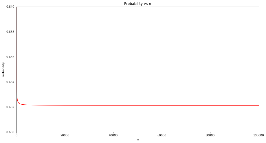
(g) Create a plot that displays, for each integer value of n from 1 to 100, 000, the probability that the jth observation is in the bootstrap sample. Comment on what you observe.
Sol: The plot is displayed below. It can be observed that for a value of n=30, the value of probability reaches around 0.632.
import numpy as np
import matplotlib.pyplot as plt

def compute_probability(n):
    return 1 - (1 - 1/n)**n

n_array = np.arange(1,100001)
prob = {}
for n in n_array:
    prob[n] = compute_probability(n)

lists = sorted(prob.items())
x, y = zip(*lists)

fig = plt.figure(figsize=(15,8))
ax = fig.add_subplot(111)
plt.plot(x, y, color='r')
ax.set_xlabel('n')
ax.set_ylabel('Probability')
ax.set_title('Probability vs n')
ax.set_xlim(10, 100000)
ax.set_ylim(0.63, 0.64)

plt.show()