A random variable is discrete if its possible values form a discrete set. The random variable denoting the experiment of rolling a fair die is an example of discrete random variable.
Let us look at an extensive example of a discrete RV. Instead of rolling a single die, we roll two fair dice. Rather than looking at the die individually, we can instead look at the sum of the dice, which would be a random variable. This is a classic example of a discrete random variable. The possible outcomes of the mentioned experiment is shown below.
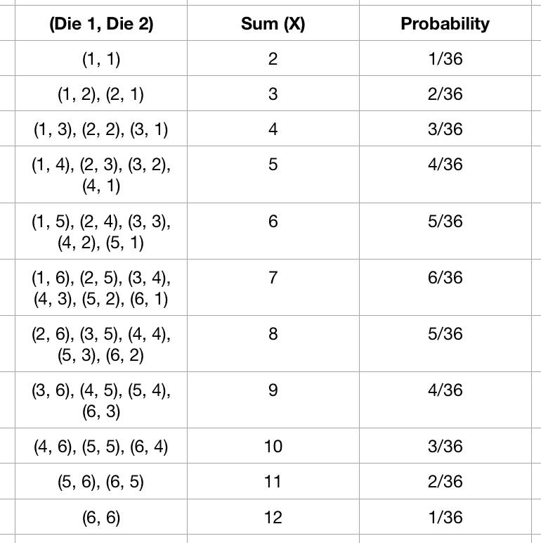
We can associate a probability with distinct values of a random variable. For example, the probability that the sum (denoted by a RV named $X$) will be equal to 6 can be written as $P(X=6)$ and is equal to $\frac{5}{36}$.
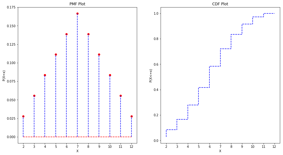
#### Probability Mass Function (PMF) :Probability mass function of a discrete random variable $X$ is the function that gives the probability that a discrete random variable is exactly equal to some value. It is denoted as $p(x) = P(X=x)$. It is also sometimes called as probability distribution. The values in the third column (named as probability) in the above table gives the PMF for the above menntioned experiment. Let us plot the PMF for the sum obtained when two fair dice is rolled. It is shown in the left plot of the below figure. The value of the RV having the highest probability mass is called the mode (7 in this case).
import matplotlib.pyplot as plt
import numpy as np

X = [2, 3, 4, 5, 6, 7, 8, 9, 10, 11, 12]
pmf = [1/36, 2/36, 3/36, 4/36, 5/36, 6/36, 5/36, 4/36, 3/36, 2/36, 1/36]
cdf = [1/36, 3/36, 6/36, 10/36, 15/36, 21/36, 26/36, 30/36, 33/36, 35/36, 36/36]

fig = plt.figure(figsize=(15,8))

# Plot of PMF
ax = fig.add_subplot(121)
plt.stem(X, pmf, linefmt='b--', markerfmt='ro', basefmt='r--')

ax.set_xlabel('X')
ax.set_ylabel('P(X=x)')
ax.set_title('PMF Plot')
plt.xticks(np.arange(min(X), max(X)+1, 1.0))

# Plot of CDF
ax = fig.add_subplot(122)
plt.step(X, cdf, color='b', linestyle='dashed')
ax.set_xlabel('X')
ax.set_ylabel('P(X<=x)')
ax.set_title('CDF Plot')
plt.xticks(np.arange(min(X), max(X)+1, 1.0))

plt.show()
 #### Cumulative Distribution Function (Discrete RV) :
Cumulative distribution function specifies the probability that a random variable is less than or equal to a given value. It can be defined as $F(x) = P(X \leq x)$. Mathematically, it can be given as:
$$F(x) = \sum_{t \leq x} p(t) = \sum _{t \leq x} P(X=t)$$
For the above experiment, $F(4) = P(X \leq 4) = \frac{1}{36} + \frac{2}{36} + \frac{3}{36} = \frac{1}{6}$. The plot of CDF is shown in the right plot of the above figure.
#### Mean and Variance of Discrete RV :The mean of a random variable $X$, which is also called as expected value and can be denoted as $\mu_X$ or $E(X)$, is given as:
$$\mu_X = \sum _{x} xP(X=x)$$
where the sum is over all possible values of $X$. The variance of a discrete random variable $X$ is the weighted average of the squared differences $(x - \mu_X)^2$, where $x$ ranges through all the possible values of RV $X$. It is given as:
$$\sigma_X^2 = \sum _{x} (x - \mu_X)^2 P(X=x)$$
The standard deviation is the square root of the variance. The code for finding the mean, variance and standard deviation for the mentioned experiment is shown below.
import math

np_X = np.array(X)
np_pmf = np.array(pmf)
mean = int(round(np.sum(np_X*np_pmf)))
print("Mean of the RV X is: " + str(mean))

(np_X - mean)**2
variance = np.sum(((np_X - mean)**2)*np_pmf)
print("Variance of the RV X is: " + str(variance))

print("Standard Deviation of the RV X is: " + str(math.sqrt(variance)))
Mean of the RV X is: 7
Variance of the RV X is: 5.833333333333334
Standard Deviation of the RV X is: 2.41522945769824
https://www.mheducation.com/highered/product/statistics-engineers-scientists-navidi/M0073401331.html