5.6 Mixture Density Networks
The goal of supervised learning is to model a conditional distribution $p(t|X)$ which for many simple regression problems is chosen to be Gaussian. However, practical machine learning problems can often have significantly non-Gaussian distributions. The main problem arises when we have to solve the inverse problem.
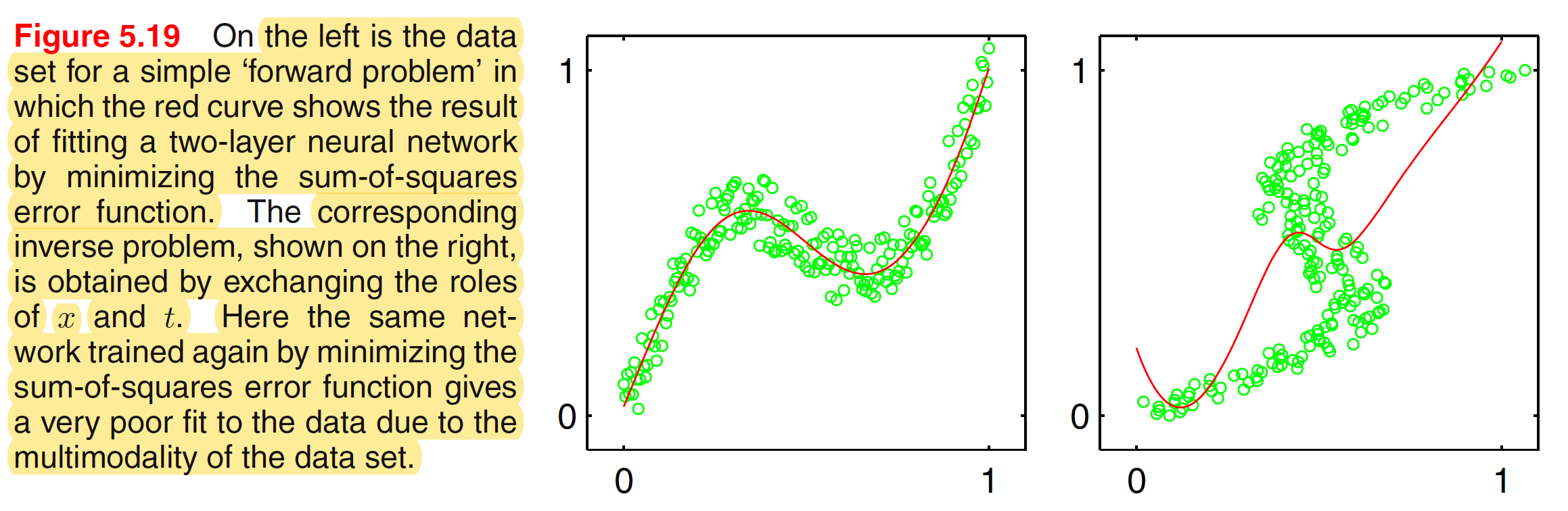
Forward problems often corresponds to causality in a physical system and generally have a unique solution. For instance, a specific pattern of symptoms in the human body may be caused by the presence of a particular disease. In pattern recognition, however, we typically have to solve an inverse problem, such as trying to predict the presence of a disease given a set of symptoms. If the forward problem involves a many-to-one mapping, then the inverse problem will have multiple solutions. For instance, several different diseases may result in the same symptoms. When the underlying distribution is multimodal, the inverse problem is more difficult to solve making the solution less obvious. The effect is shown in the below figure.
We therefore seek a general framework for modelling conditional probability distributions. This can be achieved by using a mixture model for $p(t|X)$ in which both the mixing coefficients as well as the component densities are flexible functions of the input vector $X$, giving rise to the mixture density network. For any given value of $X$, the mixture model provides a general formalism for modelling an arbitrary conditional density function $p(t|X)$. When using the Gaussian components, the resultant model is given as
$$\begin{align} p(t|X) = \sum_{k=1}^{K} \pi_k(X) N(t|\mu_k(X), \sigma_k^2(X)) \end{align}$$
The various parameters of the mixture model, namely the mixing coefficient $\pi_k(X)$, the means $\mu_k(X)$ and the variances $\sigma_k^2(X)$ are governed by the outputs of a conventional neural network that takes $X$ as its input.
The mixing component must satisfty the constraints
$$\begin{align} \sum_{k=1}^{K} \pi_k(X) = 1 \end{align}$$
where $0 \leq \pi_k(X) \leq 1$ for all values of $k$. This can be achieved using a softmax activation function at the output as
$$\begin{align} \pi_k(X) = \frac{exp(a_k^{\pi})}{\sum_{l=1}^{K}exp(a_l^{\pi})} \end{align}$$
where $a_k^{\pi}$ are the output unit activations for $\pi_k(X)$.
Variances must satisfy $\sigma_k^2(X) \geq 0$ and hence can be represented in terms of the exponentials of the corresponding network actications as
$$\begin{align} \sigma_k(X) = exp(a_k^\sigma) \end{align}$$
The means $\mu_k(X)$ has real components and hence they can be represented directly by the network output activations
$$\begin{align} \mu_k(X) = a_k^\mu \end{align}$$
The adaptive parameters of the mixture density network comprise the vector $W$ of weights and biases in the neural network, that can be set by maximum likelihood, equivalently by minimizing an error function defined to be the negative logarithm of the likelihood. For independent data, this error function takes the form
$$\begin{align} E(W) = -\sum_{n=1}^{N} \ln \bigg[ \sum_{k=1}^{K} \pi_k(X_n,W) N\big(t_n|\mu_k(X_n,W), \sigma^2_k(X_n,W)\big)\bigg] \end{align}$$
This error function can be minimized by computing the derivatives of $E(W)$ with respect to the components of $W$, which can be evaluated by using the standard backpropagation procedure.
5.7 Bayesian Neural Networks
So far, our discussion of neural networks has focussed on the use of maximum likelihood to determine the network parameters (weights and biases). Regularized maximum likelihood can be interpreted as a MAP (maximum posterior) approach in which the regularizer can be viewed as the logarithm of a prior parameter distribution.
For the Bayesian treatment of neural networks, in the case of a multilayered network, the highly nonlinear dependence of the network function on the parameter values means that an exact Bayesian treatment can no longer be found. In fact, the log of the posterior distribution will be nonconvex, corresponding to the multiple local minima in the error function. Instead, we can use Laplace approximation to approximate the posterior distribution by a Gaussian, centered at the mode of the true Gaussian. We shall also assume that the covariance of this Gaussian is small so that the network function is approximately linear with respect to the parameters over the region of parameter space for which the posterior probability is significantly nonzero.
5.7.1 Posterior Parameter Distribution
Consider the problem of predicting a single continuous target variable $t$ from a vector $X$ of inputs. Let the consitional distribution $p(t|X)$ is Gaussian, with an $X$-dependent mean given by the output $y(X,W)$ of a neural network with precison $\beta$
$$\begin{align} p(t|X,W,\beta) = N(t|y(X,W), \beta^{-1}) \end{align}$$
Let the prior distribution over the weight $W$ is Gaussian of the form
$$\begin{align} p(W| \alpha) = N(W|0, \alpha^{-1}I) \end{align}$$
For $N$ i.i.d. data set with input $X_1,X_2,…,X_N$ and corresponding set of target values $D={t_1, t_2,…,t_N}$, the likelihood function is given as
$$\begin{align} p(D|W,\beta) = \prod_{n=1}^N N(t_n|y(X_n,W), \beta^{-1}) \end{align}$$
and hence the resulting posterior distribution over the weights is
$$\begin{align} p(W|D,\alpha, \beta) \propto p(W|\alpha) p(D|W,\beta) \end{align}$$
which, as a consequence of non-linear dependence of $y(X,W)$ on $W$ will be non-Gaussian.
We can find a Gaussian approximation to the posterior distribution by using the Laplace approximation. To do this, we must first find a (local) maximum of the posterior, and this must be done using iterative numerical optimization. As usual, it is convenient to maximize the logarithm of the posterior, which can be written in the form
$$\begin{align} (- \ln p(W|D,\alpha, \beta)) = -\frac{\alpha}{2} W^TW - \frac{\beta}{2}\sum_{n=1}^{N}[y(X_n,W) - t_n]^2 + const \end{align}$$
This corrsponds to a regularixed sum-of-squares error function. Let the maximum of the posterior is found as $W_{MAP}$. To build the Gaussian approximation, we further need the second derivatives of the negative log posterior, which is given as
$$\begin{align} A = - \nabla \nabla \ln p(W|D,\alpha, \beta) = \alpha I + \beta H \end{align}$$
where $H$ is the Hessian matrix comprising the second derivatives of the sum-of-squares error function with respect to the components of $W$. The corresponding Gaussian approximation of the posterior is then given as
$$\begin{align} q(W|D) = N(W|W_{MAP}, A^{-1}) \end{align}$$
The predictive distribution can then be obtained by marginalizing with respect to this posterior distribution as
$$\begin{align} p(t|X,D) = \int p(t|X,W,\beta)q(W|D)dW \end{align}$$
Even with the Gaussian approximation of posterior, the integration is intractable due to the nonlinearity of $y(X,W)$ with respect to $W$. However, we can we now assume that the posterior distribution has small variance compared with the scales of $W$ over which $y(X,W)$ is varying. This allows us to make a Taylor series expansion of the network function around $W_{MAP}$ and retain only the linear terms as
$$\begin{align} y(X,W) \simeq y(X,W_{MAP}) + g^T(W-W_{MAP}) \end{align}$$
where
Hence, $p(t|X,W,\beta)$ can be approximated as
$$\begin{align} p(t|X,W,\beta) \simeq N(t|y(X,W_{MAP}) + g^T(W-W_{MAP}), \beta^{-1}) \end{align}$$
Hence, the predictive distribution is given as
$$\begin{align} p(t|X,D) = \int N\bigg(t|y(X,W_{MAP}) + g^T(W-W_{MAP}), \beta^{-1}\bigg) N\bigg(W|W_{MAP}, A^{-1}\bigg) dW \end{align}$$
Using the results from [https://amitrajan012.github.io/post/pattern-recognition-chapter-2-probability-distributions_5/], the marginal distribution will have the mean $y(X,W_{MAP}) + g^T(W_{MAP}-W_{MAP}) = y(X,W_{MAP})$ and variance $\beta^{-1} + g^TA^{-1}g$. Hence, the predictive distribution is a Gaussian with mean as $y(X,W_{MAP})$.
5.7.2 Bayesian Neural Networks for Classification
The above results for the regression problem can be modified and applied to the classification problenm as well. Let us consider a network having a single logistic sigmoid output for a two-class classification problem. The log likelihood for this model is then given as
$$\begin{align} \ln p(D|W) = \sum_{n} \big[t_n\ln(y_n) + (1-t_n)\ln(1-y_n)\big] \end{align}$$
where $t_n \in {0,1}$ and $y_n = y(X_n,W)$.
The first stage in applying the Laplace framework to this model is to initialize the hyperparameter $\alpha$, and then to determine the parameter vector $W$ by maximizing the log posterior distribution. This is equivalent to minimizing the regularized error function
$$\begin{align} E(W) = -\ln p(D|W) + \frac{\alpha}{2}W^TW \end{align}$$
and can be achieved using error backpropagation combined with standard optimization algorithm.
Having found a solution $W_{MAP}$ for the weight vector, the next step is to evaluate the Hessian matrix $H$ comprising the second derivatives of the negative log likelihood function.
To optimize the hyperparameter $\alpha$, we have to maximize the marginal likelihood $p(D|\alpha)$. The marginal likelihood can be given as
$$\begin{align} p(D|\alpha) = \int p(D|W,\beta) p(W|\alpha) dW \end{align}$$
Let $f(W) = p(D|W,\beta) p(W|\alpha)$, then using the results of [https://amitrajan012.github.io/post/pattern-recognition-chapter-4-linear-models-for-classification_9/], the normalizing coefficients of $f(W)$ which is equal to $\ln p(D|\alpha)$ is given as
$$\begin{align} p(D|\alpha) = f(W_{MAP})\frac{(2\pi)^{W/2}}{|A|^{1/2}} = p(D|W_{MAP},\beta) p(W_{MAP}|\alpha)\frac{(2\pi)^{W/2}}{|A|^{1/2}} \end{align}$$
where $A$ is a $W \times W$ Hessian matrix defined as
Hence,
$$\begin{align} p(D|\alpha) = \frac{(2\pi)^{W/2}}{|A|^{1/2}} p(D|W_{MAP},\beta) N(W_{MAP}|0,\alpha^{-1}I) \end{align}$$
Taking logarithm, we have
$$\begin{align} \ln p(D|\alpha) = -\frac{1}{2} \ln(|A|) + \ln [p(D|W_{MAP},\beta)] - \frac{\alpha}{2}W_{MAP}^TW_{MAP} + \frac{W}{2} \ln(\alpha) + const \end{align}$$
$$\begin{align} \ln p(D|\alpha) = -\frac{1}{2} \ln(|A|) - E(W_{MAP}) + \frac{W}{2} \ln(\alpha) + const \end{align}$$
where
$$\begin{align} E(W_{MAP}) = -\ln p(D|W_{MAP}) + \frac{\alpha}{2}W_{MAP}^TW_{MAP} \end{align}$$
$$\begin{align} E(W_{MAP}) = - \sum_{n} \big[t_n\ln(y_n) + (1-t_n)\ln(1-y_n)\big] + \frac{\alpha}{2}W_{MAP}^TW_{MAP} \end{align}$$
where $y_n = y(X_n,W_{MAP})$. This marginal log likelihood can be maximized to find the optimal value of $\alpha$.