5.5 Regularization in Neural Networks
The number of input and outputs units in a neural network is generally determined by the dimensionality of the data set, whereas the number $M$ of hidden units is a free parameter that can be adjusted to give the best predictive performance. Note that $M$ controls the number of parameters (weights and biases) in the network, and so we might expect that in a maximum likelihood setting there will be an optimum value of $M$ that gives the best generalization performance. One approach is to choose a relatively large value for $M$ and then to control complexity by the addition of a regularization term to then error function. A quadratic regularizer is given as
$$\begin{align} \tilde{E}(W) = E(W) + \frac{\lambda}{2}W^TW \end{align}$$
This regularizer is also called as weight decay. The effective model complexity is then determined by the choice of the regularization coefficient $\lambda$.
5.5.1 Consistent Gaussian Priors
One of the limitations of weight decay is it’s inconsistency with certain scaling property of network. To illustrate this, consider a multilayer perceptron network having two layers of weights and linear output units, which performs a mapping from a set of input variables ${X_i}$ to a set of output variables ${y_k}$.
The activations of the hidden units in the first hidden layer and the output layer takes the form
$$\begin{align} z_j = h\bigg(\sum_{i} W_{ji}X_i + W_{j0}\bigg) \end{align}$$
$$\begin{align} y_k = \sum_{j} W_{kj}z_j + W_{k0} \end{align}$$
Now, let us consider the case when the input is linearrly transformed as
$$\begin{align} X_i \to \tilde{X}_i = a X_i + b \end{align}$$
To keep the network mapping unchanged for this transformation, the new output of each of the layers should be same as the older one. i.e.

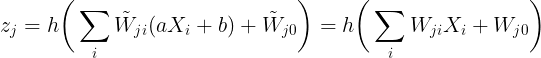
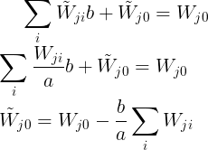
Equating the coefficients, we have

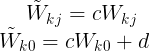
For the case when the output is linearrly transformed as
$$\begin{align} y_k \to \tilde{y}_k = cy_k + d \end{align}$$
the transformation of weights and bias of the output layer to keep the output of the network unchanged is
If we train one network using the original data and one network using data for which the input and/or target variables are transformed by one of the above linear transformations, then consistency requires that we should obtain equivalent networks that differ only by the linear transformation of the weights as given.
The regularizer which is invariant to these weight and bias transformations are given as
$$\begin{align} \frac{\lambda_1}{2} \sum_{W \in W_1} W^2 + \frac{\lambda_2}{2} \sum_{W \in W_2} W^2 \end{align}$$
where $W_1$ denotes the set of weights in the first layer,$W_2$ denotes the set of weights in the second layer, and biases are excluded from the summations. This regularizer will remain unchanged under the weight transformation provided the regularization parameters are re-scaled as $\lambda_1 \to a^{1/2}\lambda_1$ and $\lambda_2 \to c^{-1/2}\lambda_2$.
The regularizer of these types corresponds to a prior of the form
$$\begin{align} p(W|\lambda_1, \lambda_2) \propto exp\bigg(-\frac{\lambda_1}{2} \sum_{W \in W_1} W^2 - \frac{\lambda_2}{2} \sum_{W \in W_2} W^2\bigg) \end{align}$$
The priors of this form are improper (they cannot be normalized) because the bias parameters are unconstrained.
5.5.2 Early Stopping
The training of nonlinear network models corresponds to an iterative reduction of the error function defined with respect to a set of training data. For many of the optimization algorithms used for network training, the error is a nonincreasing function of the iteration index. However, the error measured with respect to independent data, generally called a validation set, often shows a decrease at first, followed by an increase as the network starts to over-fit. Training can therefore be stopped at the point of smallest error with respect to the validation data set. Halting training before a minimum of the validation error has been reached then represents a way of limiting the effective network complexity. This is called as early stopping. In the case of a quadratic error function, we can verify this insight, and show that early stopping should exhibit similar behaviour to regularization using a simple weight-decay term.
5.5.3 Invariances
In many applications of pattern recognition, it is known that predictions should be unchanged, or invariant, under one or more transformations of the input variables. If sufficiently large numbers of training patterns are available, then an adaptive model such as a neural network can learn the invariance, at least approximately. This involves including within the training set a sufficiently large number of examples of the effects of the various transformations. Thus, for translation invariance in an image, the training set should include examples of objects at many different positions. This approach may be impractical, however, if the number of training examples is limited, or if there are several invariants. We therefore seek alternative approaches for encouraging an adaptive model to exhibit the required invariances. These can broadly be divided into four categories:
-
The training set is augmented using replicas of the training patterns, transformed according to the desired invariances.
-
A regularization term is added to the error function that penalizes changes in the model output when the input is transformed. This leads to the technique of tangent propagation.
-
Invariance is built into the pre-processing by extracting features that are invariant under the required transformations. Any subsequent regression or classification system that uses such features as inputs will necessarily also respect these invariances.
-
The final option is to build the invariance properties into the structure of a neural network. One way to achieve this is through the use of local receptive fields and shared weights, as discussed in the context of convolutional neural networks.
Approach 1 is relatively easy to implement. For sequential training algorithms, this can be done by transforming each input pattern before it is presented to the model so that, if the patterns are being recycled, a different transformation is added each time. The use of such augmented data can lead to significant improvements in generalization, although it can also be computationally costly.
Approach 3 has several advantages. One advantage is that it can correctly extrapolate well beyond the range of transformations included in the training set. However, it can be difficul to find hand-crafted features with the required invariances that do not also discard information that can be useful for discrimination.
5.5.4 Tangent Propagation
We can use regularization to encourage models to be invariant to transformations of the input through the technique of tangent propagation. Consider the effect of a transformation on a particular input vector $X_n$. Provided the transformation is continuous, then the transformed pattern will sweep out a manifold $M$ within the $D$-dimensional input space. This is illustrated in the following figure for a $2$-dimensional space.

Let the transformation is governed by a parameter $\xi$ and the resultant tranformed vector is denoted as $s(X_n,\xi)$, which is defined such that $s(X,0) = X$. The tangent vector at the point $X_n$ is given as
$$\begin{align} \tau_n = \frac{\partial s(X_n,\xi)}{\partial \xi}\bigg|_{\xi=0} \end{align}$$
Under a transformation of the input vector, the network output vector will, in general, change. The derivative of output $k$ with respect to $\xi$ is given by
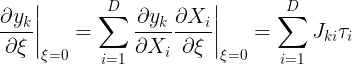
where $J_{ki}$ is the element of Jacobian matrix $J$. This can be used to modify the standard error function, so as to encourage local invariance in the neighbourhood of the data points, by the addition to the original error function $E$ of a regularization function $\Omega$, which penalizes any deviation in the predicted output $y_k$ due to the transformation, to give a total error function of the form
$$\begin{align} \tilde{E} = E + \lambda \Omega \end{align}$$
where

It can be viewed as penalizing every point $n$ in every output dimension $k$ for the transformation of the input in every possible dimension $D$.
5.5.5 Convolutional Networks
Another approach to creating models that are invariant to certain transformation of the inputs is to build the invariance properties into the structure of a neural network. This is the basis for the convolutional neural network. For example, when training on image data, a simple neural network architecture ignores a key property of images, which is that nearby pixels are more strongly correlated than more distant pixels. Many of the modern approaches to computer vision exploit this property by extracting local features that depend only on small subregions of the image. Information from such features can then be merged in later stages of processing in order to detect higher-order features and ultimately to yield information about the image as whole.
These notions can be incorporated into convolutional neural networks through three mechanisms:
- Local receptive fields
- Weight sharing
- Subsampling
In the convolutional layer the units are organized into planes, each of which is called a feature map. Units in a feature map each take inputs only from a small subregion of the image, and all of the units in a feature map are constrained to share the same weight values. For example, a feature map might consist of 100 units arranged in a $10 \times 10$ grid, with each unit taking inputs from a $5 \times 5$ pixel patch of the image. The whole feature map therefore has $25$ adjustable weight parameters plus one adjustable bias parameter. Input values from a patch are linearly combined using the weights and the bias, and the result transformed by a sigmoidal nonlinearity. If we think of the units as feature detectors, then all of the units in a feature map detect the same pattern but at different locations in the input image. Due to the weight sharing, the evaluation of the activations of these units is equivalent to a convolution of the image pixel intensities with a ‘kernel’ comprising the weight parameters. If the input image is shifted, the activations of the feature map will be shifted by the same amount but will otherwise be unchanged. Because we will typically need to detect multiple features in order to build an effective model, there will generally be multiple feature maps in the convolutional layer, each having its own set of weight and bias parameters.
The outputs of the convolutional units form the inputs to the subsampling layer of the network. For each feature map in the convolutional layer, there is a plane of units in the subsampling layer and each unit takes inputs from a small receptive fiel in the corresponding feature map of the convolutional layer. These units perform subsampling. For instance, each subsampling unit might take inputs from a $2 \times 2$ unit region in the corresponding feature map and would compute the average of those inputs, multiplied by an adaptive weight with the addition of an adaptive bias parameter, and then transformed using a sigmoidal nonlinear activation function.
The final layer of the network would typically be a fully connected, fully adaptive layer, with a softmax output nonlinearity in the case of multiclass classification.
Finally, the network can be trained by error minimization using backpropagation to evaluate the gradient of the error function. This involves a slight modificatio of the usual backpropagation algorithm to ensure that the shared-weight constraints are satisfied.
5.5.6 Soft Weight Sharing
One way to reduce the effective complexity of a network with a large number of weights is to constrain weights within certain groups to be equal. Here we consider a form of soft weight sharing in which the hard constraint of equal weights is replaced by a form of regularization in which groups of weights are encouraged to have similar values. Furthermore, the division of weights into groups, the mean weight value for each group, and the spread of values within the groups are all determined as part of the learning process.
The simple weight decay regularizer (Gaussian priors) can be viewed as the negative log of a Gaussian prior distribution over the weights. We can encourage the weight values to form several groups, rather than just one group, by considering instead a probability distribution that is a mixture of Gaussians. The centres and variances of the Gaussian components, as well as the mixing coefficients, will be considered as adjustable parameters to be determined as part of the learning process. Hence, we have a probability density of the form
$$\begin{align} p(W) = \prod_{i} p(W_i) \end{align}$$
where
$$\begin{align} p(W_i) = \sum_{j=1}^{M} \pi_j N(W_i|\mu_j,\sigma_j^2) \end{align}$$
where $\pi_j$ are mixing coefficients. Taking the negative logarithm leads to a regularization function of the form
$$\begin{align} \Omega(W) = -\ln p(W) = -\sum_{i} \ln \bigg(\sum_{j=1}^{M} \pi_j N(W_i|\mu_j,\sigma_j^2)\bigg) \end{align}$$
where the updated error function is given as
$$\begin{align} \tilde{E}(W) = E(W) + \lambda \Omega(W) \end{align}$$
This error is minimized both with respect to the weights $W_i$ and paramters ${\pi_j, \mu_j, \sigma_j}$ of the mixture model. To minimize the total error function, it is necessary to be able to evaluate its derivatives with respect to the various adjustable parameters. To do this it is convenient to regard the $\pi_j$ as prior probabilities and to introduce the corresponding posterior probabilities which, are given by Bayes’ theorem in the form
$$\begin{align} \gamma_j(W) = \frac{\pi_j N(W|\mu_j,\sigma_j^2)}{\sum_k \pi_k N(W|\mu_k,\sigma_k^2)} \end{align}$$
Taking the derivative of the error function $\tilde{E}(W)$ with respect to $W_i$, we have
$$\begin{align} \frac{\partial \tilde{E}}{\partial W_i} = \frac{\partial E}{\partial W_i} + \lambda \frac{\partial \Omega(W)}{\partial W_i} \end{align}$$
While computing the partial derivative of $\Omega(W)$ with respect to $W_i$, all the other terms apart from the one with $W_i$ in the first summation will vanish. This gives
$$\begin{align} \frac{\partial \Omega(W)}{\partial W_i} = - \frac{\partial \ln \bigg(\sum_{j=1}^{M} \pi_j N(W_i|\mu_j,\sigma_j^2)\bigg)}{\partial W_i} \end{align}$$
$$\begin{align} \frac{\partial \Omega(W)}{\partial W_i} = - \frac{1}{\sum_{j=1}^{M} \pi_j N(W_i|\mu_j,\sigma_j^2)} \sum_{j=1}^{M} \pi_j \frac{\partial N(W_i|\mu_j,\sigma_j^2)}{\partial W_i} \end{align}$$
$$\begin{align} \frac{\partial \Omega(W)}{\partial W_i} = - \frac{1}{\sum_{j=1}^{M} \pi_j N(W_i|\mu_j,\sigma_j^2)} \sum_{j=1}^{M} \pi_j N(W_i|\mu_j,\sigma_j^2) \bigg(-\frac{W_i - \mu_j}{\sigma_j^2} \bigg) \end{align}$$
$$\begin{align} \frac{\partial \Omega(W)}{\partial W_i} = \sum_{j=1}^{M} \gamma_j(W_i) \frac{W_i - \mu_j}{\sigma_j^2} \end{align}$$
Hence,
$$\begin{align} \frac{\partial \tilde{E}}{\partial W_i} = \frac{\partial E}{\partial W_i} + \lambda \sum_{j=1}^{M} \gamma_j(W_i) \frac{W_i - \mu_j}{\sigma_j^2} \end{align}$$
The effect of the regularization term is therefore to pull each weight towards the centre of the $j^{th}$ Gaussian, with a force proportional to the posterior probability of that Gaussian for the given weight.
Similarly, the derivatives of the error with respect to the centres of the Gaussians $\mu_j$ are computed as
$$\begin{align} \frac{\partial \tilde{E}}{\partial \mu_j} = \lambda \sum_{i} \gamma_j(W_i) \frac{\mu_i - W_j}{\sigma_j^2} \end{align}$$
Here, it should be noted that we have to sum over all the $i$s and while taking the derivative of the inside summation, only the one with $j$ should be considered as we are taking the derivative with respect to $\mu_j$. This derivative has a simple intuitive interpretation, because it pushes $\mu_j$ towards an average of the weight values, weighted by the posterior probabilities that the respective weight parameters were generated by component $j$.
The derivative with respect to variance can be computed similarly as
$$\begin{align} \frac{\partial \tilde{E}}{\partial \sigma_j} = \lambda \sum_{i} \gamma_j(W_i) \bigg(\frac{1}{\sigma_j} - \frac{(W_i - \mu_j)^2}{\sigma_j^3}\bigg) \end{align}$$