2.3.8 Periodic Variables
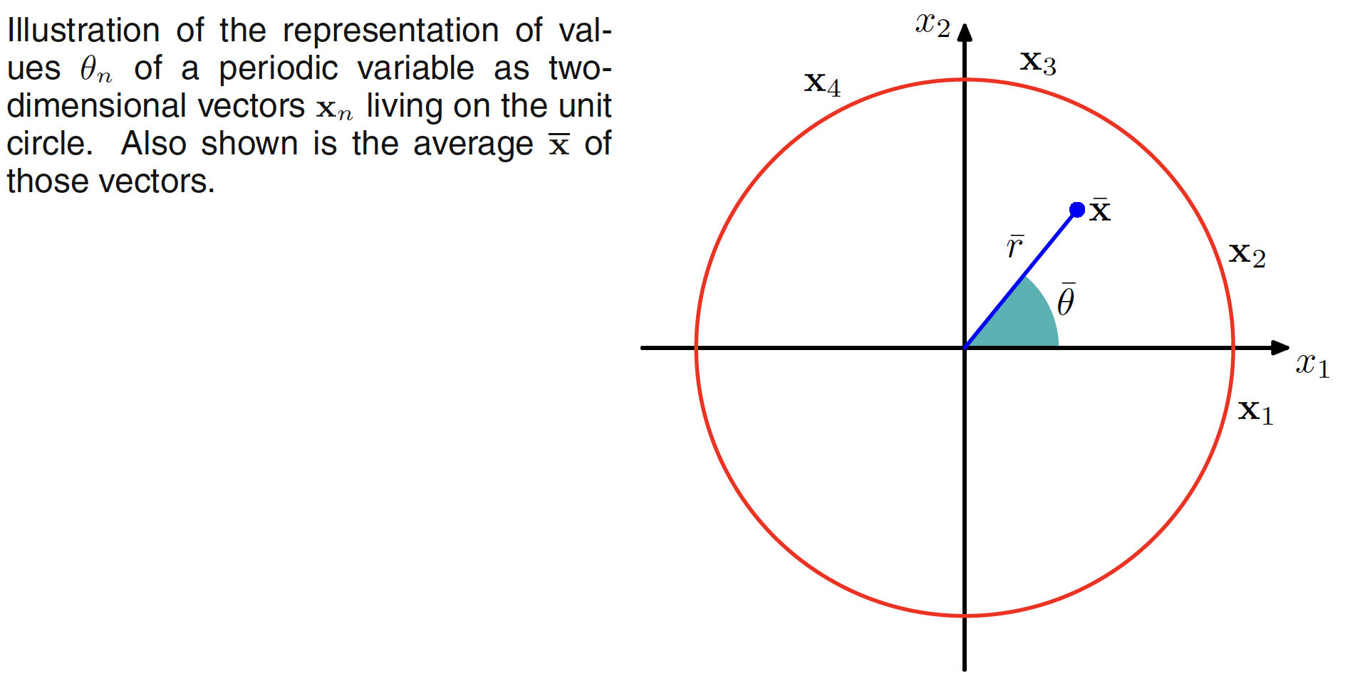
Periodic variables usually repeats its behaviour after a set amount of time. Let us assume a periodic variable represented as an angle from the x-axis by $D={\theta_1, \theta_2, …, \theta_N}$, where $\theta$ is measured in radians. The mean and variance of these data points will depend on the choice of origin and the axis. To find the invariant measure of the mean, we denote these observations as the points on the unit circle and can be described as a two-dimensional unit vectors $X_1,X_2,…,X_N$ where $||X_n|| = 1$ for $n=1,2,…,N$ as shown in the following figure.
Mean in the new coordinate system is given as
$$\begin{align} \bar{X} = \frac{1}{N}\sum_{n=1}^{N}X_n \end{align}$$
which can be used to find the mean $\bar{\theta}$. $\bar{x}$ will typically lie inside the unit circle. The coordinates of the observation are given as $X_n = (\cos \theta_n, \sin \theta_n)$ and let the coordinates of the sample mean $\bar{x}$ are $X_n = (\bar{r}\cos \bar{\theta}, \bar{r}\sin \bar{\theta})$. Then
$$\begin{align} \bar{r}\cos \bar{\theta} = \frac{1}{N}\sum_{n=1}^{N}\cos\theta_n \end{align}$$
$$\begin{align} \bar{r}\sin \bar{\theta} = \frac{1}{N}\sum_{n=1}^{N}\sin\theta_n \end{align}$$
Using these equations, we get
$$\begin{align} \bar{\theta} = \tan^{-1} \bigg(\frac{\sum_{n}\sin\theta_n}{\sum_{n}\cos\theta_n}\bigg) \end{align}$$
Periodic generaization of Gaussian is called as von Mises distribution. Let us consider a distribution $p(\theta)$ which has a period $2\pi$. $p(\theta)$ must satisfy these three conditions
$$\begin{align} p(\theta) \geq 0 \end{align}$$
$$\begin{align} \int_{0}^{2\pi} p(\theta)d\theta = 1 \end{align}$$
$$\begin{align} p(\theta + M2\pi) = p(\theta) \end{align}$$
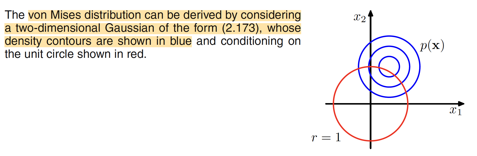
Now consider a Gaussian distribution over two variables $x=(x_1,x_2)$ having mean $\mu=(\mu_1,\mu_2)$ and a covarince matrix $\Sigma = \sigma^2I$, then
$$\begin{align} p(x_1,x_2) = \frac{1}{2\pi\sigma^2}exp\bigg[ -\frac{(x_1-\mu_1)^2+(x_2-\mu_2)^2}{2\sigma^2}\bigg] \end{align}$$
The contours of constant $p(x)$ will be circle as shown by blue concentric circles in the following figure. If we consider the value of this distribution along a circle of fixed radius, it will be periodic but not normalized.
The distribution can be transformed to polar coordiates as $x_1 = r\cos\theta$, $x_2 = r\sin\theta$ and $\mu_1 = r_0\cos\theta_0$,$\mu_2 = r_0\sin\theta_0$. The exponent in the Gaussia then reduces to
$$\begin{align} -\frac{(r\cos\theta-r_0\cos\theta_0)^2+(r\sin\theta-r_0\sin\theta_0)^2}{2\sigma^2} = \frac{r_0}{\sigma^2}\cos(\theta-\theta_0) + const \end{align}$$
Taking $m=r_0/\sigma^2$, the distribution of $p(\theta)$ along the unit circel $r=1$ is given as
$$\begin{align} p(\theta|\theta_0,m) = \frac{1}{2\pi I_0(m)} exp [m\cos(\theta - \theta_0)] \end{align}$$
and is called as von Mises distribution or circular normal distribution. $\theta_0$ correspond to the mean of the distribution and $m$ is called as the concentartion parameter and is analogous to variance. The normalization coefficient is given as
$$\begin{align} I_0(m) = \frac{1}{2\pi} \int_{0}^{2\pi} exp [m\cos\theta] d\theta \end{align}$$
The maximum likelihood estimator for the parameter $\theta_0$ and $m$ can be derived the same way. Conside the log likelihood function
$$\begin{align} \ln p(D|\theta_0,m) = - N\ln(2\pi) - N\ln I_0(m) + m\sum_{n=1}^{N}\cos(\theta_n - \theta_0) \end{align}$$
Setting the derivative with respect to $\theta_0$ equal to $0$, we get
$$\begin{align} \sum_{n=1}^{N}\sin(\theta_n - \theta_0) = 0 \end{align}$$
Solving this equation, we get
$$\begin{align} \theta_0^{ML} = \tan^{-1}\bigg[\frac{\sum_n\sin\theta_n}{\sum_n\cos\theta_n} \bigg] \end{align}$$
2.3.9 Mixtures of Gaussians
Linear combination of Gaussians can give rise to very complex densities. By using a sufficient number of Gaussians, and by adjusting their means and covariances as well as the coefficients in the linear combination, almost any continuous density can be approximated to arbitrary accuracy. Superposition of $K$ Gaussians of the form
$$\begin{align} p(X) = \sum_{k=1}^{K} \pi_{k} N(X|\mu_k, \Sigma_k) \end{align}$$
is called as mixture of Gaussians. Each Gaussian $N(X|\mu_k, \Sigma_k)$ is called as the component of the mixture and has its own mean and variance. The parameters $\pi_k$ are called mixing coefficicnts such that $0 \leq \pi_k \leq 1$ and should satisfy
$$\begin{align} \sum_{k=1}^{K}\pi_k = 1 \end{align}$$