2.3.6 Bayesian Inference for the Gaussian
We can use Bayesian treatment to derive the point estimates for the mean and variance of the Gaussian by introducing prior distributions over these parameters. For a single ranodm variable, let us suppose that the variance $\sigma^2$ is known and we have to determine the mean $\mu$ given $N$ data points $X={x_1,x_2,…,x_N}$. Under the assumption of independence, the likelihood function is give as
$$\begin{align} p(X|\mu) = \prod_{n=1}^{N} p(x_n|\mu) = \frac{1}{(2\pi\sigma^2)^{N/2}} exp \bigg(-\frac{1}{2\sigma^2}\sum_{n=1}^{N}(x_n - \mu)^2\bigg) \end{align}$$
As the likelihood function takes the form of the exponential of a quadratic form in $\mu$, we can choose a conjugate prior $p(\mu)$ given by the Gaussian as
$$\begin{align} p(\mu) = N(\mu|\mu_0, \sigma_0^2) \end{align}$$
Posterior distribution is given as
$$\begin{align} p(\mu|X) \propto p(X|\mu)p(\mu) \end{align}$$
$$\begin{align} p(\mu|X) \propto exp \bigg(-\frac{1}{2\sigma^2}\sum_{n=1}^{N}(x_n - \mu)^2\bigg)exp \bigg(-\frac{1}{2\sigma_0^2}(\mu - \mu_0)^2\bigg) \end{align}$$
$$\begin{align} p(\mu|X) \propto exp \bigg(\sum_{n=1}^{N}\bigg[-\frac{1}{2\sigma^2}(x_n - \mu)^2 -\frac{1}{2N\sigma_0^2}(\mu - \mu_0)^2\bigg]\bigg) \end{align}$$
The quadratic form can be completed as
$$\begin{align} \sum_{n=1}^{N}\bigg[-\frac{1}{2\sigma^2}(x_n - \mu)^2 -\frac{1}{2N\sigma_0^2}(\mu - \mu_0)^2\bigg] \end{align}$$
$$\begin{align} =\sum_{n=1}^{N}\bigg[-\frac{1}{2\sigma^2}(x_n^2 + \mu^2 - 2x_n\mu) -\frac{1}{2N\sigma_0^2}(\mu^2 + \mu_0^2 - 2\mu\mu_0)\bigg] \end{align}$$
$$\begin{align} =\sum_{n=1}^{N}-\frac{1}{2}\bigg[\bigg(\frac{1}{\sigma^2} + \frac{1}{N\sigma_0^2}\bigg)\mu^2 - 2\bigg(\frac{x_n}{\sigma^2} + \frac{\mu_0}{N\sigma_0^2}\bigg)\mu+ const\bigg] \end{align}$$
$$\begin{align} =-\frac{1}{2}\bigg[\bigg(\frac{N}{\sigma^2} + \frac{1}{\sigma_0^2}\bigg)\mu^2 - 2\bigg(\sum_{n=1}^{N}\frac{x_n}{\sigma^2} + \frac{\mu_0}{\sigma_0^2}\bigg)\mu+ const\bigg] \end{align}$$
$$\begin{align} =-\frac{1}{2}\bigg[\bigg(\frac{N}{\sigma^2} + \frac{1}{\sigma_0^2}\bigg)\mu^2 - 2\bigg(\frac{N\mu_{ML}}{\sigma^2} + \frac{\mu_0}{\sigma_0^2}\bigg)\mu + const\bigg] \end{align}$$
Comparing the above expression with the generic quadratic form of Gaussian shown below, we can compute the mean and variance.
$$\begin{align} \Delta^2 = -\frac{1}{2}(X-\mu)^T\Sigma^{-1}(X-\mu) = -\frac{1}{2}X^T\Sigma^{-1}X + X^T\Sigma^{-1}\mu + const \end{align}$$
Coefficient of second order term gives us the inverse of variance, i.e.
$$\begin{align} \frac{1}{\sigma_N^2} = \frac{1}{\sigma_0^2} + \frac{N}{\sigma^2} \end{align}$$
The coefficient of first order term gives us the product of mean and inverse of varince, i.e.
$$\begin{align} \frac{\mu_N}{\sigma_N^2} = \frac{N\mu_{ML}}{\sigma^2} + \frac{\mu_0}{\sigma_0^2} \end{align}$$
$$\begin{align} \mu_N = \sigma_N^2 \bigg(\frac{N\mu_{ML}}{\sigma^2} + \frac{\mu_0}{\sigma_0^2}\bigg) = \frac{\sigma_0^2\sigma^2}{\sigma^2+N\sigma_0^2} \bigg(\frac{N\mu_{ML}}{\sigma^2} + \frac{\mu_0}{\sigma_0^2}\bigg) \end{align}$$
$$\begin{align} \mu_N = \frac{\sigma^2}{\sigma^2+N\sigma_0^2}\mu_0 + \frac{N\sigma_0^2}{\sigma^2+N\sigma_0^2}\mu_{ML} \end{align}$$
where
$$\begin{align} \mu_{ML} = \frac{1}{N}\sum_{n=1}^{N}x_n \end{align}$$
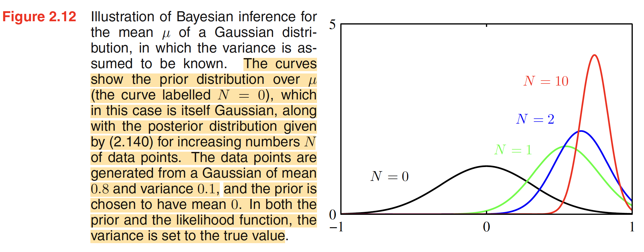
The mean $\mu_N$ of the postrior distribution is a compromise between prior mean and MLE mean. If $N = 0$, it reduces to prior mean and as $N \to \infty$, the posterior mean is given by the maximum likelihood mean $\mu_{ML}$. If we look at the expression for inverse of the varince, i.e. precision, precison of the posterior is given by the precision of the prior plus one contribution of the data precision from each of the observed data points. Precision steadily increases which means that the variance steadily decreases as we see more and more data points. As $N \to \infty$, $\sigma_N^2 \to 0$ and hence the posterior distribution infinitely peaks around the maximum likelihood solution. Bayesian inference of mean is illustrated in the following figure.
Bayesian inference leads natrually to a sequential estimation process as the estimate of the mean can be expressed as follown.
$$\begin{align} p(\mu|D) \propto \bigg[p(\mu)\prod_{n=1}^{N-1}p(x_n|\mu)\bigg]p(x_N|\mu) \end{align}$$
The term in square bracket is the posterior distribution upto observing $N-1$ data points. This can be viewed as a prior distribution for $N^{th}$ data point which when combined with the likelihood function of $N^{th}$ data point (given as $p(x_N|\mu)$) gives us the posterior distribution after observing $N$ data points.
2.3.7 Student’s t-distribution
Student’s t-distribution is defined as
$$\begin{align} St(x|\mu,\lambda,v) = \frac{\Gamma(v/2+1/2)}{\Gamma(v/2)} \bigg(\frac{\lambda}{\pi v}\bigg)^{1/2} \bigg[ 1 + \frac{\lambda(x-\mu)^2}{v}\bigg]^{-v/2-1/2} \end{align}$$
The parameter $v$ is called as the degree of freedom and its effect is illustrated in following figure. As $v\to\infty$, the t-distribution reduces to a Gaussian $N(x|\mu,\lambda^{-1})$ with mean $\mu$ and precision $\lambda$.
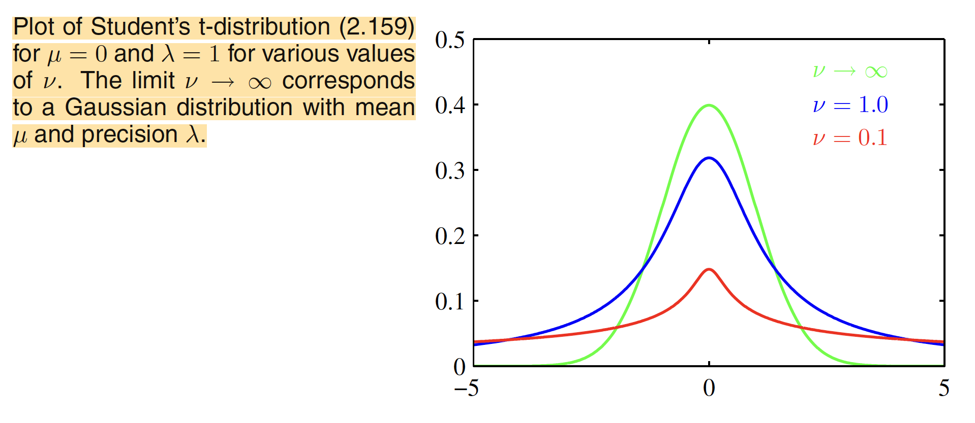
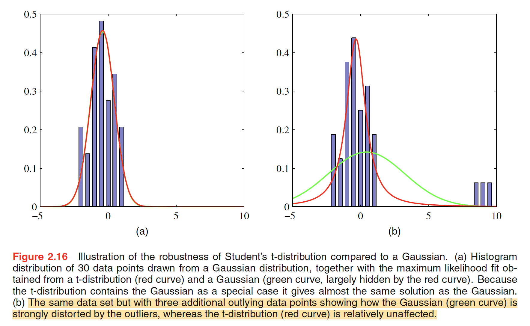
Student’s t-distribution is obtained by adding up an infinite number of Gaussian distributions having the same mean but different precisions. This can be interpreted as an infinite mixture of Gaussians.The result is a distribution that in general has longer ‘tails’ than a Gaussian, as seen in the above figure. This gives the tdistribution an important property called robustness, which means that it is much less sensitive than the Gaussian to the presence of a few data points which are outliers. Robustness to outliers withe example is shown in the following figure.