For $X_1, X_2, …, X_n$ be a large ($n > 30$) random sample from a population with mean $\mu$ and standard deviation $\sigma$, so that $\overline{X}$ is approximately normal (from Central Limit Theorem). Then a level $100(1- \alpha)%$ confidence interval of $\mu$ is
$$\overline{X} \pm z _{\alpha/2} \sigma _{\overline{X}}$$
where $\sigma_{\overline{X}} = \frac{\sigma}{\sqrt{n}}$. When the value of population standard deviation $\sigma$ is unknown, it can be replaced with the sample standard deviation $s$.
Example: The sample mean and standard deviation for the fill weights of 100 boxes are $\overline{X} = 12.05$ and $s = 0.1$. Find an 85% confidence interval for the mean fill weight of the boxes.
Sol: First of all, $1 - \alpha = 85%$, and hence $\frac{\alpha}{2} = .075$. From the z-table, the z-value corresponding to $0.075$ is 1.44. Hence, the confidence interval is
$$12.05 \pm 1.44 (\frac{0.1}{\sqrt{100}}) = 12.05 \pm 0.0144 = (12.0356, 12.0644)$$
Let us design an experiment to understand the meaning of confidence interval in deep. A random data set is generated (treated as population) and 100 random samples of size 1000 are drawn from it and 68%, 95.6% and 99.7% confidence interval for the population mean is computed. The experimental results are well in accordance with the theoretical values.
import random
import numpy as np

random.seed(1)

X = np.array(random.sample(range(1, 100000), 10000))/100000
population_mean = X.mean()

# Generate 100 random samples
count_68 = 0
count_96 = 0
count_99 = 0
for i in range(1000):
    S = np.random.choice(X, size=100, replace=True)
    # Compute 68% confidene interval
    lower = S.mean() - S.std()/10
    upper = S.mean() + S.std()/10
    if (lower <= population_mean and population_mean <= upper):
        count_68 += 1
    # Compute 95% confidene interval
    lower = S.mean() - 1.96*S.std()/10
    upper = S.mean() + 1.96*  S.std()/10
    if (lower <= population_mean and population_mean <= upper):
        count_96 += 1
    # Compute 99.7% confidene interval
    lower = S.mean() - 3*S.std()/10
    upper = S.mean() + 3*  S.std()/10
    if (lower <= population_mean and population_mean <= upper):
        count_99 += 1
print("The percentage of time the 68% confidence interval covers the population mean is: " +str(count_68/10)+"%")
print("The percentage of time the 95.6% confidence interval covers the population mean is: " +str(count_96/10)+"%")
print("The percentage of time the 99.7% confidence interval covers the population mean is: " +str(count_99/10)+"%")
The percentage of time the 68% confidence interval covers the population mean is: 68.0%
The percentage of time the 95.6% confidence interval covers the population mean is: 95.1%
The percentage of time the 99.7% confidence interval covers the population mean is: 99.7%
Sometimes it is required to find the sample size needed for a confidence interval to be of specified width. The needed sample size can be calculated as shown in the below example.
Example: In an experiment, the sample standard deviation of weights from 100 boxes was s = 0.1 oz. How many boxes must be sampled to obtain a 99% confidence interval of width ±0.012 oz?
Sol: For a 99% confidence interval, $\alpha = 0.01$, and hence $z _{\alpha/2} = z _{0.005} = 2.58$. Given, $s= 0.1$ and hence, the required equation is
$$\frac{2.58 \times 0.1}{\sqrt{n}} = 0.012$$
which gives $n \approx 463$.
Sometimes one-sided confidence interval is desirable. The $100(1-\alpha)%$ one sided confidence interval can be calculated as:
$$Lower \ bound = \overline{X} - z _{\alpha}\sigma _{\overline{X}}$$
$$Upper \ bound = \overline{X} + z _{\alpha}\sigma _{\overline{X}}$$
where $\sigma _{\overline{X}} = \frac{\sigma}{\sqrt{n}}$ and the value of $\sigma$ can be estimated from sample standard deviation $s$.
It should be noted that the method described above is based on the fact that the data is a random sample from the population. If this condition is violated, the above explained method does not hold true.
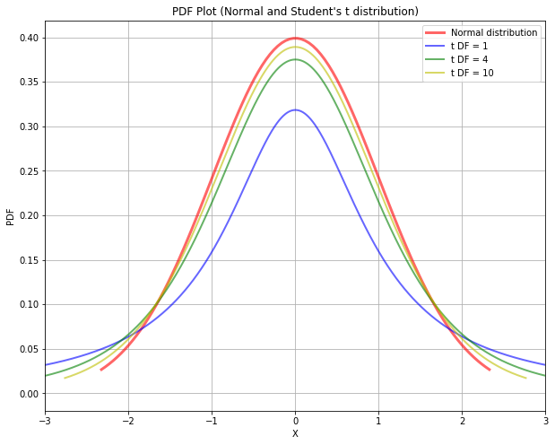
#### Confidence Intervals for a Population Mean (Small-Sample) :For a small sample size, there is no generic method to find the confidence interval for the population mean. However, when the population is approximately normal, a probability distribution called as the Student’s t distribution can be used to compute confidence intervals for the population mean. The plot of probability density functions for various Student’s t distribution is shown below. The shape of the PDF of Student’s t distribution is same as that of the normal distribution but the spread is more. For a sample size of $n$, the degree of freedom of Student’s t distribution is $n-1$. As the degree of freedom (or the sample size) increases, the shape of Student’s t distribution approximates normal distribution. The plot of Student’s t distribution with $df=30$ will be almost indistinguishable from the normal PDF plot.
from scipy.stats import t
from scipy.stats import norm
import matplotlib.pyplot as plt

fig = plt.figure(figsize=(10,8))
# Plot of PDF of normal distribution
ax = fig.add_subplot(111)
x = np.linspace(norm.ppf(0.01), norm.ppf(0.99), 100)
ax.plot(x, norm.pdf(x, scale=1), 'r-', lw=3, alpha=0.6, label='Normal distribution')

# Plot of PDF of Student's t distribution
df = 1
x = np.linspace(t.ppf(0.01, df), t.ppf(0.99, df), 10000)
ax.plot(x, t.pdf(x, df), 'b-', lw=2, alpha=0.6, label='t DF = 1')

# Plot of PDF of Student's t distribution
df = 4
x = np.linspace(t.ppf(0.01, df), t.ppf(0.99, df), 10000)
ax.plot(x, t.pdf(x, df), 'g-', lw=2, alpha=0.6, label='t DF = 4')

# Plot of PDF of Student's t distribution
df = 10
x = np.linspace(t.ppf(0.01, df), t.ppf(0.99, df), 10000)
ax.plot(x, t.pdf(x, df), 'y-', lw=2, alpha=0.6, label='t DF = 10')

ax.set_xlabel('X')
ax.set_ylabel('PDF')
ax.set_xlim(-3, 3)
ax.set_title("PDF Plot (Normal and Student's t distribution)")
ax.legend()
ax.grid()

plt.show()
Let $X_1, X_2, …, X_n$ be a small sample ($n < 30$) from a normal population with mean $\mu$. The quantity
$$\frac{\overline{X} - \mu}{s/\sqrt{n}}$$
will have a Student’s t distribution with $n-1$ degree of freedoms, denoted as $t_{n-1}$. For large value of $n$, the distribution of above quantity is close to normal and hence the normal curve can be used. Hence, a $100(1-\alpha)%$ confidence interval for $\mu$ can be given as:
$$\overline{X} \pm t_{n-1, \alpha/2} \frac{s}{\sqrt{n}}$$
It should be noted that the essential condition for the application of Student’s t distribution while computing the confidence interval is the fact that sample comes from a population that is approximately normal. The one-sided confidence interval can be given as:
$$Lower \ bound = \overline{X} - t_{n-1, \alpha}\frac{s}{\sqrt{n}}$$
$$Upper \ bound = \overline{X} + t_{n-1, \alpha}\frac{s}{\sqrt{n}}$$
One reason to use Student’s t distribution while computing the confidence interval is the fact that the population standard deviation $\sigma$ is unknown and hence is approximated by sample standard deviation $s$. When population standard deviation $\sigma$ is known, normal distribution (z-table) is used instead for the computation of the confidence interval.
#### Reference :https://www.mheducation.com/highered/product/statistics-engineers-scientists-navidi/M0073401331.html