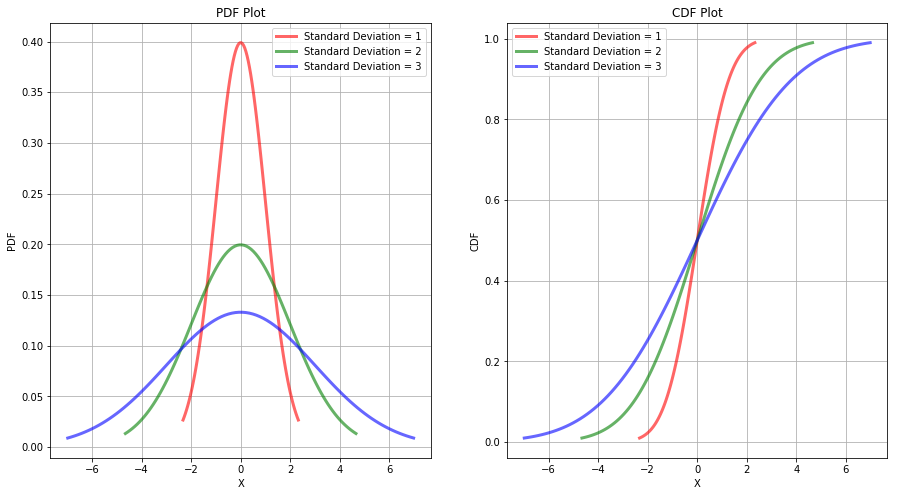
The normal distribution is a continuous distribution with any mean and a positive variance. The probability density function of a normal distribution with mean $\mu$ and variance $\sigma^2$ is given as:
$$f(x) = \frac{1}{\sigma \sqrt{2\pi}} e^{-\frac{(x-\mu)^2}{2\sigma^2}}$$
The above normal distribution is denoted as $X \sim N(\mu, \sigma^2)$ with mean and variance as:
$$\mu_X = \mu$$
$$\sigma_X^2 = \sigma^2$$
For a normal distribution, about 68% of the population is in the interval $\mu \pm \sigma$, 95% in $\mu \pm 2\sigma$ and 99.7% in $\mu \pm 3\sigma$. It is a widespread practice to convert the units of the normal population to the standard units which tells us that how many standard deviations an observation is from the population mean. It is sometimes called as z-score and is given as:
$$z = \frac{x-\mu}{\sigma}$$
z-score can also be viewed as an item sampled from a normal distribution with mean 0 and standard deviation 1, which is called as the standard normal population. As normal distribution is a continuous distribution, to calculate the probabilities we need to find the area under the curve and hence need to do the integration of the normal density function. But the integration of the normal density funaction can not be found by the use of elementary calculus and hence the area under the standard normal curve is extensively tabulated and is called as standard normal table or z table.
The parameters of a normal distribution can be estimated from the sample mean and sample standard deviation. The estimate of population mean $\mu$ is the sample mean $\overline{X}$. Sample variance $s^2$ gives the estimate of population variance $\sigma^2$. Sample mean is the unbiased estimator of population mean with an uncertainty of $\frac{\sigma}{\sqrt{n}}$.
If $X$ is a normal random variable with distribution $N(\mu, \sigma^2)$, the distribution of $aX+b$ is given as:
$$N(a\mu+b, a^2 \sigma^2)$$
For independent and normally distributed random variables $X_1, X_2, …, X_n$, with means $\mu_1, \mu_2, …, \mu_n$ and variances $\sigma_1^2, \sigma_2^2, …, \sigma_n^2$ and constants $c_1, c_2, …, c_n$, the distribution of the linear combination $c_1X_1 + c_2X_2 + … + c_nX_n$ is given as:
$$N(c_1\mu_1 + c_2\mu_2 + … + c_n\mu_n, c_1^2\sigma_1^2 + c_2^2\sigma_2^2 + … + c_n^2\sigma_n^2)$$
For a better understanding, the plot of PDF and CDF of a normal distribution is shown below.
import numpy as np
from scipy.stats import norm
import matplotlib.pyplot as plt

fig = plt.figure(figsize=(15,8))

# Plot of PMF
ax = fig.add_subplot(121)
x = np.linspace(norm.ppf(0.01), norm.ppf(0.99), 100)
ax.plot(x, norm.pdf(x, scale=1), 'r-', lw=3, alpha=0.6, label='Standard Deviation = 1')

x = np.linspace(norm.ppf(0.01, scale=2), norm.ppf(0.99, scale=2), 100)
ax.plot(x, norm.pdf(x, scale=2), 'g-', lw=3, alpha=0.6, label='Standard Deviation = 2')

x = np.linspace(norm.ppf(0.01, scale=3), norm.ppf(0.99, scale=3), 100)
ax.plot(x, norm.pdf(x, scale=3), 'b-', lw=3, alpha=0.6, label='Standard Deviation = 3')

ax.set_xlabel('X')
ax.set_ylabel('PDF')
ax.set_title('PDF Plot')
ax.legend()
ax.grid()

ax = fig.add_subplot(122)
x = np.linspace(norm.ppf(0.01), norm.ppf(0.99), 100)
ax.plot(x, norm.cdf(x, scale=1), 'r-', lw=3, alpha=0.6, label='Standard Deviation = 1')

x = np.linspace(norm.ppf(0.01, scale=2), norm.ppf(0.99, scale=2), 100)
ax.plot(x, norm.cdf(x, scale=2), 'g-', lw=3, alpha=0.6, label='Standard Deviation = 2')

x = np.linspace(norm.ppf(0.01, scale=3), norm.ppf(0.99, scale=3), 100)
ax.plot(x, norm.cdf(x, scale=3), 'b-', lw=3, alpha=0.6, label='Standard Deviation = 3')

ax.set_xlabel('X')
ax.set_ylabel('CDF')
ax.set_title('CDF Plot')
ax.legend()
ax.grid()

plt.show()
 #### The Lognormal Distribution :
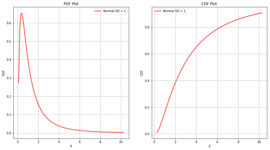
If $X$ is a normal random variable with mean $\mu$ and variance $\sigma^2$, then the random variable $Y=e^X$ is said to have a lognormal distribution with parameters $\mu$ and $\sigma^2$. Hence, $X=ln Y$ is a normal distribution with parameter $\mu$ and $\sigma^2$. The lognornmal distribution is highly skewed to the right and hence is often used to model datasets that have outliers. It should be noted that $\mu$ and $\sigma^2$ in the lognormal distribution is the mean and variance of the underlying normal distribution. The mean and variance of the lognormal distribution is given as:
$$\mu_Y = e^{(\mu + \frac{\sigma^2}{2})}$$
$$\sigma_Y^2 = e^{(2\mu + 2\sigma^2)} - e^{(2\mu + \sigma^2)}$$
To check whether the data comes from a lognormal distribution or not, we can take the natural logarithm of the data points and try to see whether they follow a normal distribution or not. For a better understanding, the plot of PDF and CDF of a lognormal distribution is shown below.
import numpy as np
from scipy.stats import lognorm
import matplotlib.pyplot as plt

fig = plt.figure(figsize=(15,8))

# Plot of PMF
ax = fig.add_subplot(121)
x = np.linspace(lognorm.ppf(0.01, s=1, scale=np.exp(0)), lognorm.ppf(0.99, s=1, scale=np.exp(0)), 100)
ax.plot(x, lognorm.pdf(x, s=1, scale=np.exp(0)), 'r-', lw=3, alpha=0.6, label='Normal SD = 1')


ax.set_xlabel('X')
ax.set_ylabel('PDF')
ax.set_title('PDF Plot')
ax.legend()
ax.grid()

ax = fig.add_subplot(122)
x = np.linspace(lognorm.ppf(0.01, s=1, scale=np.exp(1)), lognorm.ppf(0.99, s=1, scale=1), 100)
ax.plot(x, lognorm.cdf(x, s=1, scale=np.exp(1)), 'r-', lw=3, alpha=0.6, label='Normal SD = 1')

ax.set_xlabel('X')
ax.set_ylabel('CDF')
ax.set_title('CDF Plot')
ax.legend()
ax.grid()

plt.show()
 #### The Exponential Distribution :
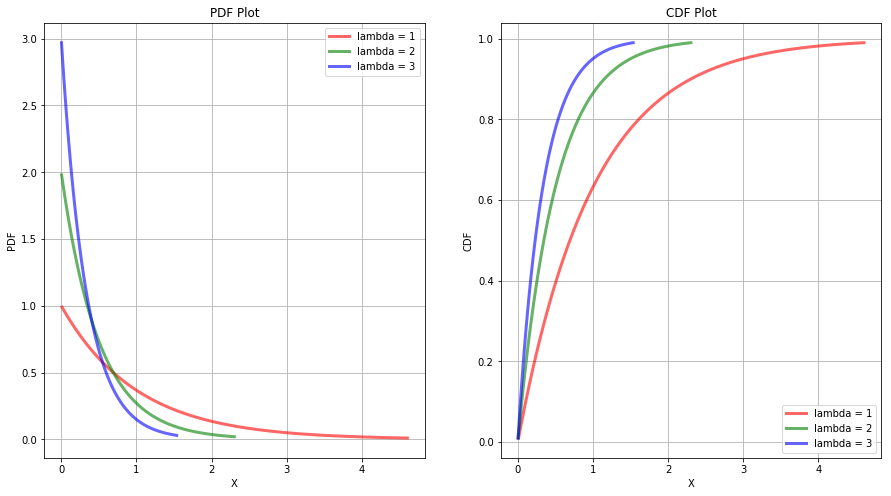
The exponential distribution is a continuous distribution that is used to model the time (called as waiting time) that elapses before an event occurs. There is a close connection between the exponential and the Poisson distribution. The probability density function of the exponential distribution with parameter $\lambda$, where $\lambda > 0$ is given as:
$$f(x) = \lambda e^{-\lambda x}$$
The cumulative distribution function of the exponential distribution can be computed as:
$$F(x) = P(X \leq x) = \int_{0}^{x} \lambda e^{-\lambda t} dt = 1 - e^{-\lambda x}$$
The mean and variance of the exponential distribution is given as:
$$\mu_X = \frac{1}{\lambda}$$
$$\sigma_X^2 = \frac{1}{\lambda^2}$$
The exponential distribution suffers from the lack of memory property. For an exponential distribution, the probability that we must wait an additional $t$ units, given that we have already waited $s$ units, is the same as the probability that we must wait $t$ units from the start. This can be shown from an example.
Example: The lifetime of a particular integrated circuit has an exponential distribution with mean 2 years. Find the probability that the circuit lasts longer than three years.
Sol: As the mean $\mu = \frac{1}{\lambda} = 2$, $\lambda = 0.5$ and hence variance $\sigma^2 = 4$. We have to find $P(T>3)$.
$$P(T>3) = 1 - P(T \leq 3) = 1 - (1 - e^{-0.5 \times 3}) = 0.223$$
Example: Assume the circuit is now four years old and is still functioning. Find the probability that it functions for more than three additional years.
Sol: Here, we have to find the conditional probability $P(T>7 \ \big| \ T>4)$.
$$P(T>7 \ \big| \ T>4) = \frac{P(T>7 \ and \ T>4)}{P(T>4)} = \frac{P(T>7)}{P(T>4)} = \frac{e^{-0.5 \times 7}}{e^{-0.5 \times 4}} = e^{-0.5 \times 3} = 0.223$$
Hence, the probability of syrviving three more years is same in both the case. This shows the lack of memory property of the exponential distribution.
For a better understanding, the plot of PDF and CDF of several exponential distributions is shown below.
import numpy as np
from scipy.stats import expon
import matplotlib.pyplot as plt

fig = plt.figure(figsize=(15,8))

# Plot of PMF
ax = fig.add_subplot(121)
x = np.linspace(expon.ppf(0.01, scale=1), expon.ppf(0.99, scale=1), 100)
ax.plot(x, expon.pdf(x, scale=1), 'r-', lw=3, alpha=0.6, label='lambda = 1')

x = np.linspace(expon.ppf(0.01, scale=1/2), expon.ppf(0.99, scale=1/2), 100)
ax.plot(x, expon.pdf(x, scale=1/2), 'g-', lw=3, alpha=0.6, label='lambda = 2')

x = np.linspace(expon.ppf(0.01, scale=1/3), expon.ppf(0.99, scale=1/3), 100)
ax.plot(x, expon.pdf(x, scale=1/3), 'b-', lw=3, alpha=0.6, label='lambda = 3')

ax.set_xlabel('X')
ax.set_ylabel('PDF')
ax.set_title('PDF Plot')
ax.legend()
ax.grid()

ax = fig.add_subplot(122)
x = np.linspace(expon.ppf(0.01, scale=1), expon.ppf(0.99, scale=1), 100)
ax.plot(x, expon.cdf(x, scale=1), 'r-', lw=3, alpha=0.6, label='lambda = 1')

x = np.linspace(expon.ppf(0.01, scale=1/2), expon.ppf(0.99, scale=1/2), 100)
ax.plot(x, expon.cdf(x, scale=1/2), 'g-', lw=3, alpha=0.6, label='lambda = 2')

x = np.linspace(expon.ppf(0.01, scale=1/3), expon.ppf(0.99, scale=1/3), 100)
ax.plot(x, expon.cdf(x, scale=1/3), 'b-', lw=3, alpha=0.6, label='lambda = 3')

ax.set_xlabel('X')
ax.set_ylabel('CDF')
ax.set_title('CDF Plot')
ax.legend()
ax.grid()

plt.show()
 #### The Uniform Distribution :
The uniform distribution (which is a continuous distribution), with parameters $a$ and $b$ is defined as:
$$f(x) = \frac{1}{b-a}, \ when\ a< x < b, \ othersise \ 0$$
The mean and variance of uniform distribution can be computed as:
$$\mu _X = \int _{-\infty}^{\infty} xf(x) \ dx = \int _{a}^{b} \frac{x}{b-a} \ dx = \frac{x^2}{b-a} \bigg|_a^b = \frac{a+b}{2}$$
$$\sigma_X^2 = E[{(x-\mu_X)^2}] = \int _{-\infty}^{\infty} (x-\mu_X)^2f(x) \ dx = \int _{a}^{b} \frac{(x-\mu_X)^2}{b-a} \ dx = \frac{(x-\mu_X)^3}{3(b-a)} \bigg|_a^b = \frac{(b- \frac{a+b}{2})^3}{3(b-a)} - \frac{(a- \frac{a+b}{2})^3}{3(b-a)} = \frac{(b- a)^2}{12}$$
#### Reference :https://www.mheducation.com/highered/product/statistics-engineers-scientists-navidi/M0073401331.html