9.4 The EM Algorithm in General
The expectation maximization (EM) algorithm is a general technique for finding maximum likelihood solutions for probabilistic models having latent variables. Consider a probabilistic model in which observed variable is denoted by $X$ and the hidden variable by $Z$. The joint distribution $p(X,Z|\theta)$ is governed by a set of parameters deonoted by $\theta$. Our goal is to maximize the likelihood function given by
$$\begin{align} p(X|\theta) = \sum_{Z} p(X,Z|\theta) \end{align}$$
For a continuous $Z$, summation is replaced by integration. Direct optimization of $p(X|\theta)$ is difficult but the optimization of comlete-data likelihood function $p(X,Z|\theta)$ is somewhat easier. A distribution $q(Z)$ over the latent variable is introduced and we observe that for any choice of $q(Z)$, following decomposition holds true.
$$\begin{align} \ln p(X|\theta) = L(q,\theta) + KL(q||p) \end{align}$$
where
$$\begin{align} L(q,\theta) = \sum_Z q(Z) \ln \bigg[ \frac{p(X,Z|\theta)}{q(Z)} \bigg] \end{align}$$
$$\begin{align} KL(q||p) = - \sum_Z q(Z) \ln \bigg[ \frac{p(Z|X, \theta)}{q(Z)} \bigg] \end{align}$$
$L(q,\theta)$ contains the joint distribution of $X,V$ while $KL(q||p)$ contains the conditional distribution of $Z$ given $X$. $KL(q||p)$ is also called as the Kullback-Liebler divergence between $q(Z)$ and the posterior distribution $p(Z|X, \theta)$. This term satisfies $KL(q||p) \geq 0$ with equality holding if and only if $q(Z) = p(Z|X, \theta)$. Hence, $\ln p(X|\theta) \geq L(q,\theta)$, which means that $L(q,\theta)$ is the lower bound of $\ln p(X|\theta)$. This is illustrated in below figure.

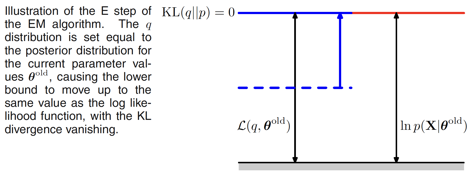
The EM algorithm is a two step process. In the E step, the current value of the parameter vector $\theta^{old}$ is used to maximize tge lower bound $L(q,\theta^{old})$ with respect to $q(Z)$. The solution to this maximization problem can be visualized as follows. The value of $\ln p(X|\theta)$ does not depend on $q(Z)$ and hence the largest value of $L(q,\theta^{old})$ will occur when the Kullback-Liebler divergence vanishes, i.e. $q(Z) = p(Z|X, \theta^{old})$. This is illustrated in following figure.
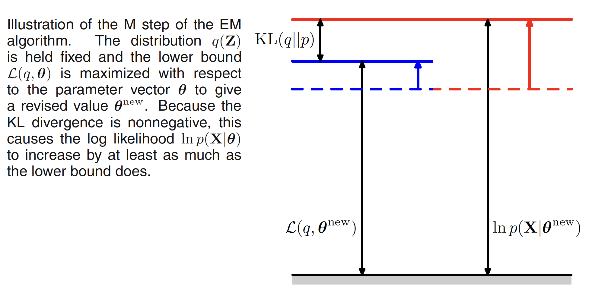
In the M step, $q(Z)$ is kept fixed and the lower bound $L(q,\theta^{old})$ is maximized with respect to $\theta$ to give some new value $\theta^{new}$. This will cause the lower bound $L$ to increase which will cause the corresponding log likelihood function to increase. As the distribution $q$ is determined using the old parameter values and is held fixed during the M step, it will not be equal to the new posterior distribution $p(Z|X, \theta^{new})$ and hence there will be nonzero KL divergence. The M step is illustrated in following figure.
The EM algorithm breaks down the potentially difficult problem of maximizing the likelihood function into two stages, the E step and the M step, each of which will often prove simpler to implement.