One of the significant limitations of learning algorithms based on non-linear kernels is that the kernel function $k(X_n, X_m)$ must be evaluated for all possible pairs $X_n$ and $X_m$ of training points. For us, it will be favourable that we shall look at kernel-based algorithms that have sparse solutions, so that predictions for new inputs depend only on the kernel function evaluated at a subset of the training data points. One of the most used sparse solution is support vector machine (SVM). An important property of support vector machines is that the determination of the model parameters corresponds to a convex optimization problem, and so any local solution is also a global optimum. It should be noted that the SVM is a decision machine and so does not provide posterior probabilities.
7.0 Lagrange Multipliers
Lagrange multipliers, also sometimes called undetermined multipliers, are used to find the stationary points of a function of several variables subject to one or more constraints. Consider the problem of finding the maximum of a function $f(x_1, x_2)$ subject to a constraint relating $x_1$ and $x_2$, which we write in the form
$$\begin{align} g(x_1, x_2) = 0 \end{align}$$
One approach is to solve $g(x_1, x_2) = 0$ to get $x_2 = h(x_1)$ and then substitute it in $f(x_1, x_2)$ to get a function of the form $f(x_1, h(x_1))$ which can then be maximized with respect to $x_1$ to get the solution $x_1^{*}$ which can be furrther used to find $x_2 = h(x_1^{*})$. The problem in this approach is that it may be difficult to find the analytical solution of $g(x_1, x_2) = 0$ to find the expression $x_2 = h(x_1)$.
A more elegant, and often simpler, approach is based on the introduction of a parameter $\lambda$ called a Lagrange multiplier. We shall motivate this technique from a geometrical perspective. Consider a $D$-dimensional variable $x$ with components $x_1,x_2,…,x_D$. The constarint equation $g(x) = 0$ then represents a $(D-1)$-dimensional surface in $x$-space as shown in below figure.
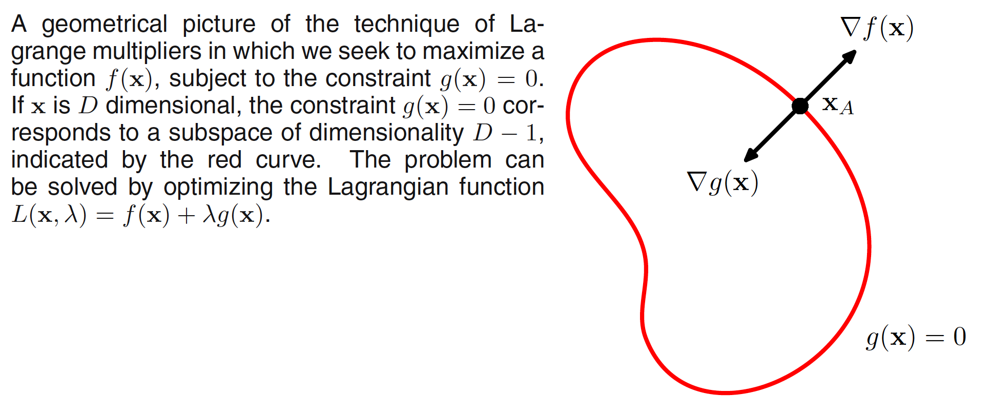
At any point on the constraint surface the gradient $\nabla g(x)$ of the constraint function will be orthogonal to the surface. To prove this, consider a point $x$ that lies on the constraint surface and also consider a nearby point $x+\epsilon$ that also lies on the surface. Taking Taylor expansion around $x$, we have
$$\begin{align} g(x+\epsilon) \simeq g(x) + \epsilon^T \nabla g(x) \end{align}$$
As both $x$ and $x+\epsilon$ lie on the surface, we have $g(x) = g(x+\epsilon)$ and hence $\epsilon^T \nabla g(x) \simeq 0$. As $\epsilon$ is parallel to $g(x)$, $\nabla g(x)$ will be perpendicular to it.
Next we seek a point $x$ on the constraint surface such that $f(x)$ is maximized. Such a point must have the property that the vector $\nabla f(x)$ is also orthogonal to the constraint surface, as illustrated in the above figure, because otherwise we could increase the value of $f(x)$ by moving a short distance along the constraint surface. Thus $\nabla f$ and $\nabla g$ are parallel (or anti-parallel) vectors, and so there must exist a parameter $\lambda$ such that
$$\begin{align} \nabla f + \lambda \nabla g = 0 \end{align}$$
where $\lambda \neq 0$ is a Lagrange multiplier. We can further introduce the Lagrangian function defined as
$$\begin{align} L(x, \lambda) = f(x) + \lambda g(x) \end{align}$$
Taking the derivative with respect to $x$ and equating it to $0$, we get the expression $\nabla f + \lambda \nabla g = 0$. The derivative with respect to $\lambda$ gives us the constraint equation $g(x) = 0$. Thus to find the maximum of a function subject to the constraint, we define the Lagrangian function and we then find the stationary point of $L(x,\lambda)$ with respect to both x and $\lambda$.
For example, suppose we wish to find the stationary point of the function $f(x_1,x_2) = 1 - x_1^2 - x_2^2$ subject to the constraint $g(x_1,x_2) = x_1 + x_2 - 1 = 0$. Corresponding Lagrangian function is given as
$$\begin{align} L(x_1, x_2, \lambda) = 1 - x_1^2 - x_2^2 + \lambda (x_1 + x_2 - 1) \end{align}$$
Taking derivatives with respect to $x_1,x_2,\lambda$ and equating them to $0$, we get
$$\begin{align} -2x_1 + 1 = 0 \end{align}$$
$$\begin{align} -2x_2 + 1 = 0 \end{align}$$
$$\begin{align} x_1 + x_2 - 1 = 0 \end{align}$$
Solving these equations, we get $x_1 = x_2 = 1/2$ which gives us the stationary point as $(1/2,1/2)$ and the Lagrangian multiplier $\lambda = 1$.
We now consider the problem of maximizing $f(x)$ subject to an inequality constraint of the form $g(x) \geq 0$, as illustrated in the below figure.
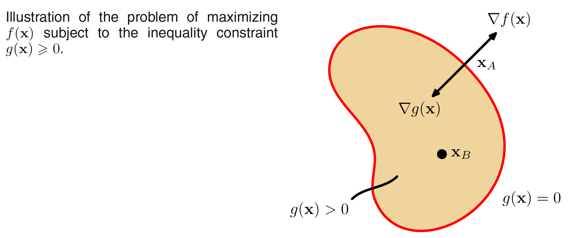
There are now two kinds of solution possible, according to whether the constrained stationary point lies in the region where $g(x) > 0$, in which case the constraint is inactive, or whether it lies on the boundary $g(x) = 0$, in which case the constraint is said to be active. In the former case, the function $g(x)$ plays no role and so the stationary condition is simply $\nabla f(x) = 0$ which corresponds to the stationary point of the Lagrange function with $\lambda = 0$. The latter case, where the solution lies on the boundary, is analogous to the equality constraint discussed previously and corresponds to a stationary point of the Lagrange function with $\lambda \neq 0$.
Now, however, the sign of the Lagrange multiplier is crucial, because the function $f(x)$ will only be at a maximum if its gradient is oriented away from the region $g(x) > 0$, as illustrated in the above figure. We therefore have $\nabla f(x) = −\lambda \nabla g(x)$ for some value of $\lambda > 0$.
For either of these two cases, the product $\lambda g(x) = 0$. Hence, the solution to the problem of maximizing $f(x)$ subject to the constratint $g(x) \geq 0$ is obtained by optimizing the Lagrange function with respect to $x,\lambda$ subject to the conditions
$$\begin{align} g(x) \geq 0 \end{align}$$
$$\begin{align} \lambda \geq 0 \end{align}$$
$$\begin{align} \lambda g(x) = 0 \end{align}$$
These are known as the Karush-Kuhn-Tucker (KKT) conditions.
Note that if we wish to minimize (rather than maximize) the function $f(x)$ subject to an inequality constraint $g(x) \geq 0$, then we minimize the Lagrangian function $L(x, \lambda) = f(x) - \lambda g(x) $ with respect to x, again subject to $\lambda \geq 0$. Finally, it is straightforward to extend the technique of Lagrange multipliers to the case of multiple equality and inequality constraints.