6.2 Constructing Kernels
One way to construct a kernel is to choose a feature space mapping $\phi(X)$ and then use this to find the corresponding kernel. Let $x$ be a one dimensional input. The kernel function is then given as
$$\begin{align} k(x,x^{’}) = \phi(x)^T\phi(x^{’}) = \sum_{i=1}^{M} \phi_i(x)\phi_i(x^{’}) \end{align}$$
where $\phi_i(x)$ are the basis functions.
An alternative approach is to construct kernel functions directly. In this case, we must ensure that the function we choose is a valid kernel, in other words that it corresponds to a scalar product in some (perhaps infinite dimensional) feature space. For example, consider a simple kernel function given as
$$\begin{align} k(X,Z) = (X^T,Z)^2 \end{align}$$
For a two dimensional input space $X=(x_1,x_2)$, the kernel function reduces to
$$\begin{align} k(X,Z) = (X^TZ)^2 = (x_1z_1 + x_2z_2)^2 = (x_1^2, \sqrt{2}x_1x_2, x_2^2)(z_1^2, \sqrt{2}z_1z_2, z_2^2)^T \end{align}$$
and hence the feature mapping takes the form $\phi(X) = (x_1^2, \sqrt{2}x_1x_2, x_2^2)^T$.
We need a simple way to test whether a function constitutes a valid kernel without having to construct the function $\phi(X)$ explicitly. A necessary and sufficient condition for a function $k(X,X^{’})$ to be a valid kernel is that the Gram matrix $K$, whose elements are given by $k(X_n,X_m)$, should be positive semidefinite for all possible choices of the set ${X_n}$.
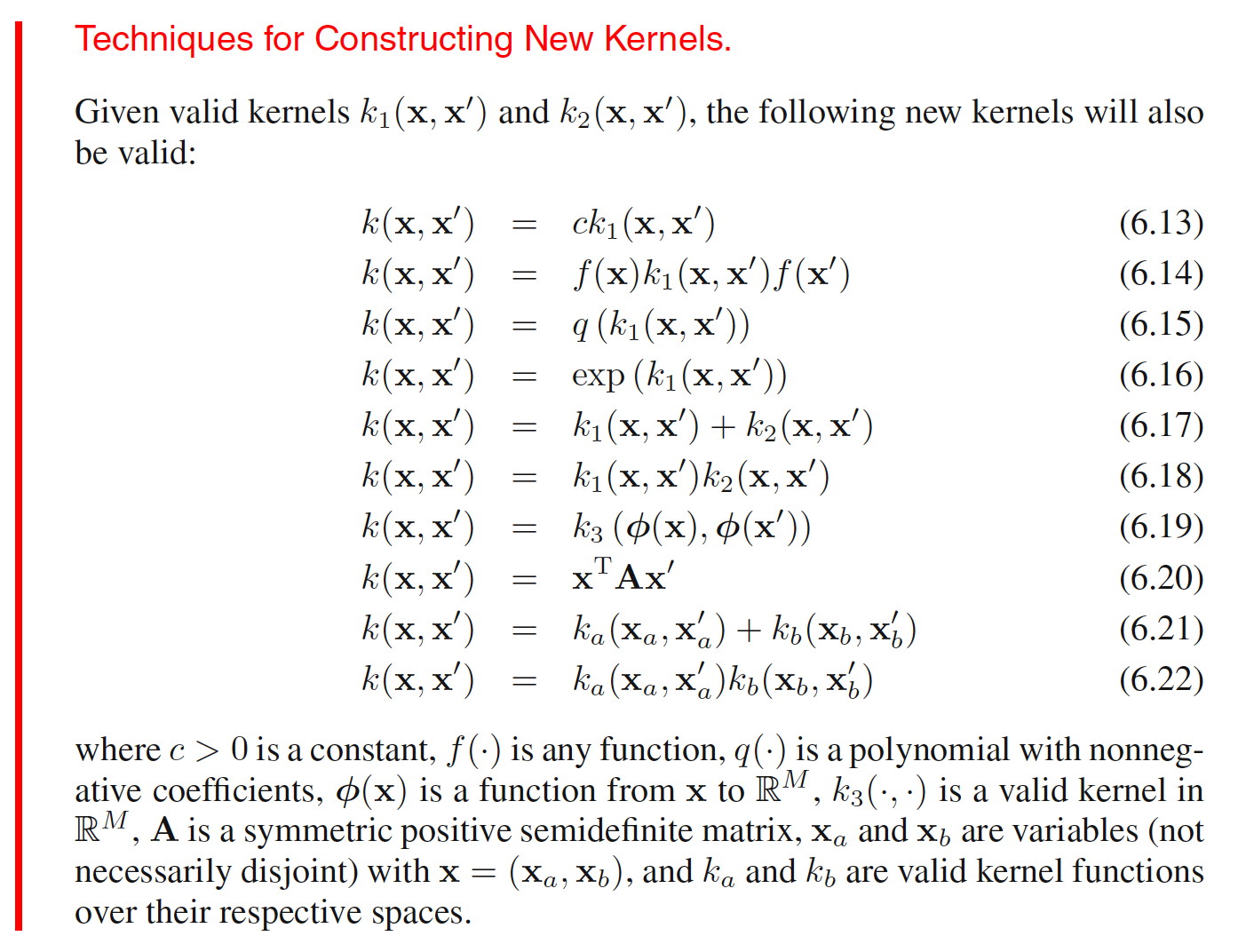
One powerful technique for constructing new kernels is to build them out of simpler kernels as building blocks.
One of the commonly used kernels is the Gaussian kernel. It takes the form
$$\begin{align} k(X,X^{’}) = \exp (-||X-X^{’}||^2/2\sigma^2) \end{align}$$
In this context, it is not interpreted as a probability density, and hence the normalization coefficient is omitted. To check whether it’s a valid kernel or not, we can expand the square and get
$$\begin{align} ||X-X^{’}||^2 = X^TX + (X^{’})^TX^{’} - 2X^TX^{’} \end{align}$$
This gives us
$$\begin{align} k(X,X^{’}) = \exp(-X^TX/2\sigma^2) \exp(-X^TX^{’}/\sigma^2) \exp(-(X^{’})^TX^{’}\sigma^2) \end{align}$$
As $X^TX^{’}$ is a valid kernerl, $-X^TX^{’}/\sigma^2$ is a valid kernel from (6.13). Applying (6.16) on it, we get $\exp(-X^TX^{’}/\sigma^2)$ as a valid kernel. Taking $f(X) = \exp(-X^TX/2\sigma^2)$ and applying (6.14), we get $k(X,X^{’})$ as a valid kernel. Note that the feature vector that corresponds to the Gaussian kernel has infinite dimensionality.
There are certail advantages and disadvantages of difference modeling techniques. Generative models can deal naturally with missing data. Discriminative models generally give better performance on discriminative tasks than generative models. There are approaches which can be used to combine them. One way to combine them is to use a generative model to define a kernel, and then use this kernel in a discriminative approach.
Given a generative model $p(X)$, we can define a kernel as
$$\begin{align} k(X,X^{’}) = p(X)p(X^{’}) \end{align}$$
This is a valid kernel function because we can interpret it as an inner product in the one-dimensional feature space defined by the mapping $p(X)$. It says that two inputs $X$ and $X^{’}$ are similar if they both have high probabilities. (6.13) and (6.17) can be used to extend this class of kernels by considering sums over products of different probability distributions, with positive weighing coefficients $p(i)$, of the form
$$\begin{align} k(X,X^{’}) = \sum_{i}p(X|i)p(X^{’}|i)p(i) \end{align}$$
Two inputs $X$ and $X^{’}$ will give a large value for the kernel function, and hence appear similar, if they have significant probability under a range of different components.
6.3 Radial Basis Function Networks
Radial basis functions have the property that each basis function depends only on the radial distance (typically Euclidean) from a centre $\mu_j$, so that $\phi_j(X) = h(||X-\mu_j||)$.
Radial basis functions were introduced for the purpose of exact function interpolation. Given a set of input vectors ${X_1, X_2, …, X_N}$ along with corresponding target values ${t_1, t_2, …, t_N}$, the goal is to find a smooth function $f(X)$ that fits every target value exactly, so that $f(X_n) = t_n$ for all $n=1,2,…,N$. This is achieved by expressing $f(X)$ as a linear combination of radial basis functions, one centred on every data point
$$\begin{align} f(X) = \sum_{n=1}^{N} w_n h(||X-X_n||) \end{align}$$
The values of the coefficiens ${w_n}$ are found by least squares, and because there are the same number of coefficients as there are constraints, the result is a function that fits every target value exactly. In pattern recognition applications, however, the target values are generally noisy, and exact interpolation is undesirable because this corresponds to an over-fitted solution.
As there is one basis function associated with every data point, the corresponding model can be computationally costly to evaluate when making predictions for new data points. Models have therefore been proposed which retain the expansion in radial basis function but where the number $M$ of basis functions is smaller than the number $N$ of data points. Typically, the number of basis functions, and the locations $\mu_j$ of their centres, are determined based on the input data ${X_n}$ alone. The basis functions are then kept fixed and the coefficient ${w_i}$ are determined by least squares by solving the usual set of linear equations. One of the simplest ways of choosing basis function centres is to use a randomly chosen subset of the data points. A more systematic approach is called orthogonal least squares. This is a sequential selection process in which at each step the next data point to be chosen as a basis function centre corresponds to the one that gives the greatest reduction in the sum-of-squares error.
6.3.1 Nadaraya-Watson Model
We can motivate the kernel regression model from a different perspective, starting with kernel density estimation. Suppose we have a training set ${X_n,t_n}$ and we use a Parzen density estimator to model the joint distribution $p(X,t)$, such that
$$\begin{align} p(X,t) = \frac{1}{N}\sum_{n=1}^{N}f(X-X_n, t-t_n) \end{align}$$
where $f(X,t)$ is the component density function, and there is one such component centred on each data point. The expression for the regression function $y(X)$ can be found as
$$\begin{align} y(X) = E[t|X] = \int_{-\infty}^{\infty} tp(t|X)dt = \int_{-\infty}^{\infty} tp(t|X)dt \end{align}$$
$$\begin{align} = \int_{-\infty}^{\infty} t\frac{p(X,t)}{p(X)}dt = \frac{\int_{-\infty}^{\infty} tp(X,t)dt}{p(X)} = \frac{\int tp(X,t)dt}{\int p(X,t)dt} \end{align}$$
$$\begin{align} = \frac{\sum_n \int t f(X-X_n, t-t_n) dt}{\sum_m \int f(X-X_m, t-t_m) dt} \end{align}$$
For simplicity, we can assume that the component density functions have $0$ mean, so that
$$\begin{align} \int_{-\infty}^{\infty} tf(X, t) dt = 0 \end{align}$$
Using change of variable as $t-t_n \to t$ and $t-t_m \to t$, we get
$$\begin{align} y(X) = \frac{\sum_n \int (t + t_n) f(X-X_n, t) dt}{\sum_m \int f(X-X_m, t) dt} \end{align}$$
$$\begin{align} = \frac{\sum_n \bigg[ \int t f(X-X_n, t) dt + \int t_n f(X-X_n, t) dt\bigg]}{\sum_m \int f(X-X_m, t) dt} \end{align}$$
$$\begin{align} = \frac{\sum_n \int t_n f(X-X_n, t) dt}{\sum_m \int f(X-X_m, t) dt} = \frac{\sum_n t_n g(X-X_n)}{\sum_m g(X-X_m)} \end{align}$$
where
$$\begin{align} g(X) = \int_{-\infty}^{\infty} f(X, t) dt \end{align}$$
Hence,
$$\begin{align} y(X) = \frac{\sum_n t_n g(X-X_n)}{\sum_m g(X-X_m)} = \sum_n t_n \frac{g(X-X_n)}{\sum_m g(X-X_m)} = \sum_n t_n k(X,X_n) \end{align}$$
where the kernel function $k(X,X_n)$ is given as
$$\begin{align} k(X,X_n) = \frac{g(X-X_n)}{\sum_m g(X-X_m)} \end{align}$$
The above result for $y(X)$ is called as Nadaraya-Watson model or kernel regression model. For a localized kernel function, it has the property of giving more weight to the data points $X_n$ that are close to $X$. The kernel satisfies the summation constraint
$$\begin{align} \sum_{n=1}^{N} k(X,X_n) = 1 \end{align}$$