4.3 Probabilistic Discriminative Models
For two-class classification problem, the posterior probability of classes are the logistic sigmoid transformation of a linear function of input $X$. For multi-class classification problem, they are given by the softmax transformation of a linear function of input $X$. In maximum likelihood solution, we chose the class-conditional densities and then maximized the log likelihood to obtain posterior densities. However, an alternative approach is to use the functional form of the generalized linear model explicitly instead and to determine its parameters directly by using maximum likelihood. In this approach, we are maximizing a likelihood function defined through the conditional distribution $p(C_k|X)$, which represents a form of discriminative function. One advantage of the discriminative approach is that there will typically be fewer adaptive parameters to be determined. Unlike generative modeling, it can not be used to generate synthetic data as we won’t have the distributions $p(X)$ and $p(X|C_k)$.
4.3.1 Fixed Basis Functions
So far, we have considered classification models that work directly with the original input vector $X$. However, all of the algorithms are equally applicable if we first make a fixed nonlinear transformation of the inputs using a vector of basis functions $\phi(X)$. The resulting decision boundaries will be linear in the feature space $\phi$, and these correspond to nonlinear decision boundaries in the original input space.
4.3.2 Logistic Regression
For a two-class classification problem, under rather general assumptions, the posterior probability of class $C_1$ can be written as a logistic sigmoid acting on a linear function of the transformed input space $\phi$ so that
$$\begin{align} p(C_1|\phi) = y(\phi) = \sigma(W^T\phi) \end{align}$$
with $p(C_2|\phi) = 1 - p(C_1|\phi)$, where $\sigma(.)$ is a logistic sigmoid function defined as
$$\begin{align} \sigma(a) = \frac{1}{1 + exp(-a)} \end{align}$$
This model is called as logistic regression. For a $M$-dimensional feature space, this model has $M$ adjustable parameters. If we have modeled the Gaussian class-conditional densities using maximum likelihood approach, we would have a total of $2M$ parameters for the class means and $M(M+1)/2$ parameters for shared covariance matrix. To use the maximum likelihood to obtain the parameters of logistic regression model, we have to compute the derivative of the logistic sigmoid function. This can be done as
$$\begin{align} \frac{d\sigma}{da} = \frac{d\sigma(a)}{da} = \frac{-1}{[1 + exp(-a)]^2}exp(-a)(-1) = \frac{exp(-a)}{[1 + exp(-a)]^2} \end{align}$$
$$\begin{align} = \frac{1}{1 + exp(-a)}\bigg[1 - \frac{1}{1 + exp(-a)}\bigg] = \sigma(a)(1 - \sigma(a)) = \sigma(1 - \sigma) \end{align}$$
For a data set ${\phi_n, t_n}$ where $\phi_n = \phi(X_n)$ for $n=1,2,…,N$ and $t_n \in {0,1}$, the likelihood function can be written as
$$\begin{align} p(t|W) = \prod_{n=1}^{N} p(C_1|\phi_n)^{t_n} p(C_2|\phi_n)^{1-t_n} = \prod_{n=1}^{N} y_n^{t_n} (1 - y_n)^{1-t_n} \end{align}$$
The error function, defined as negative log likelihhod, is given as
$$\begin{align} E(W) = -\ln p(t|W) = -\sum_{n=1}^{N} t_n \ln y_n + (1-t_n) \ln(1 - y_n) \end{align}$$
where $y_n = \sigma(W^T\phi_n)$. To compute the derivative of $E(W)$ with respect to $W$, we have to compute the derivative of $y_n$ first, which can be done as
$$\begin{align} \frac{dy_n}{dW} = \frac{d\sigma(W^T\phi_n)}{dW} = \sigma(1 - \sigma)\phi_n \end{align}$$
Hence,
$$\begin{align} \nabla E(W) = -\sum_{n=1}^{N} \frac{t_n}{y_n} \sigma(1 - \sigma)\phi_n - \frac{1 - t_n}{1 - y_n} \sigma(1 - \sigma)\phi_n \end{align}$$
$$\begin{align} = -\sum_{n=1}^{N} \sigma(1 - \sigma)\phi_n\frac{t_n - y_n}{y_n(1-y_n)} = \sum_{n=1}^{N} y_n(1 - y_n)\phi_n\frac{y_n - t_n}{y_n(1-y_n)} \end{align}$$
$$\begin{align} \nabla E(W) = \sum_{n=1}^{N} \phi_n(y_n - t_n) \end{align}$$
Hence, the contribution to the gradient from data point $n$ is given by the error $y_n - t_n$ between the target value and the prediction of the model, times the basis function vector $\phi_n$. One important thing to note is that the maximum likelihood can exhibit severe over-fitting problem for data sets that are even linearly separable.
4.3.3 Multiclass Logistic Regression
In a multi-class classification problem, posterior probability is give by a softmax transformation of linear function of feature vector as
$$\begin{align} p(C_k|\phi) = y_k(\phi) = \frac{exp(a_k)}{\sum_{j}exp(a_j)} \end{align}$$
where the activation function $a_k$ is given as
$$\begin{align} a_k = W_k^T\phi \end{align}$$
This posterior probability model can directly be maximized with respect to parameter $W_k$. To do this, we will require the derivative of $y_k$ with respect to all of $a_j$. It can be given as
$$\begin{align} \frac{\delta y_k}{\delta a_j} = \begin{cases} \frac{-exp(a_k)exp(a_j)}{[\sum_j exp(a_j)]^2} = -y_ky_j, & j \neq k\\ \frac{\sum_j exp(a_j) exp(a_k) - exp(a_k) exp(a_k)}{[\sum_j exp(a_j)]^2} = y_k[1 - y_k], & j = k \end{cases} \end{align}$$
These two equations can be combined and written as
$$\begin{align} \frac{\delta y_k}{\delta a_j} = y_k(I_{kj} - y_j) \end{align}$$
where $I_{kj}$ is the element of identity matrix. $I_{kj}$ will be $1$ when $j=k$ and $0$ otherwise. To define the likelihood function, the target vector matrix (for a total of $N$ samples and $K$ class each sample) is encoded as $T$ where for sample $n$ belonging to class $C_k$, the target vector $t_n$ will have an entry of $1$ at position $k$ and $0$ otherwise, i.e. $t_{nk} = 1$ and $t_{nj} = 0$ where $j \neq k$. The likelihood function is then given as
$$\begin{align} p(T|W_1, W_2, …, W_K) = \prod_{n=1}^{N}\prod_{k=1}^{K}p(C_k|\phi_n)^{t_{nk}} = \prod_{n=1}^{N}\prod_{k=1}^{K}y_{nk}^{t_{nk}} \end{align}$$
where $y_{nk} = y_k(\phi_n)$ and $T$ is a $N \times K$ matrix. Taking the negative logarithm, error function is given as
$$\begin{align} E(W_1,W_2,…,W_K) = -\sum_{n=1}^{N}\sum_{k=1}^{K}t_{nk}\ln(y_{nk}) \end{align}$$
which is also called as cross-entropy error function for the multiclass classification problem. Taking the derivative of error function with respect to $W_j$, we have
$$\begin{align} \nabla_{W_j}E(W_1,W_2,…,W_K) = -\sum_{n=1}^{N} (y_{nj} - t_{nj})\phi_{n} \end{align}$$
The above expression is once again the product of error and the basis function $\phi_{n}$, which is similar to the two-class case.
4.3.5 Probit Regression
For a broad range of class-conditional distributions, described by the exponential family, the resulting posterior class probabilities are given by a logistic (or softmax) transformation acting on a linear function of the feature variables. However, not all choices of class-conditional density give rise to such a simple form for the posterior probabilities. Let a genralized linear model take the form
$$\begin{align} p(t=1|a) = f(a) \end{align}$$
where $a=W^T\phi$ and $f(.)$ is activation function. We can design the activation function as
$$\begin{align} \begin{cases} t_n = 1, & a_n \geq \theta\\ t_n = 0, & otherwise \end{cases} \end{align}$$
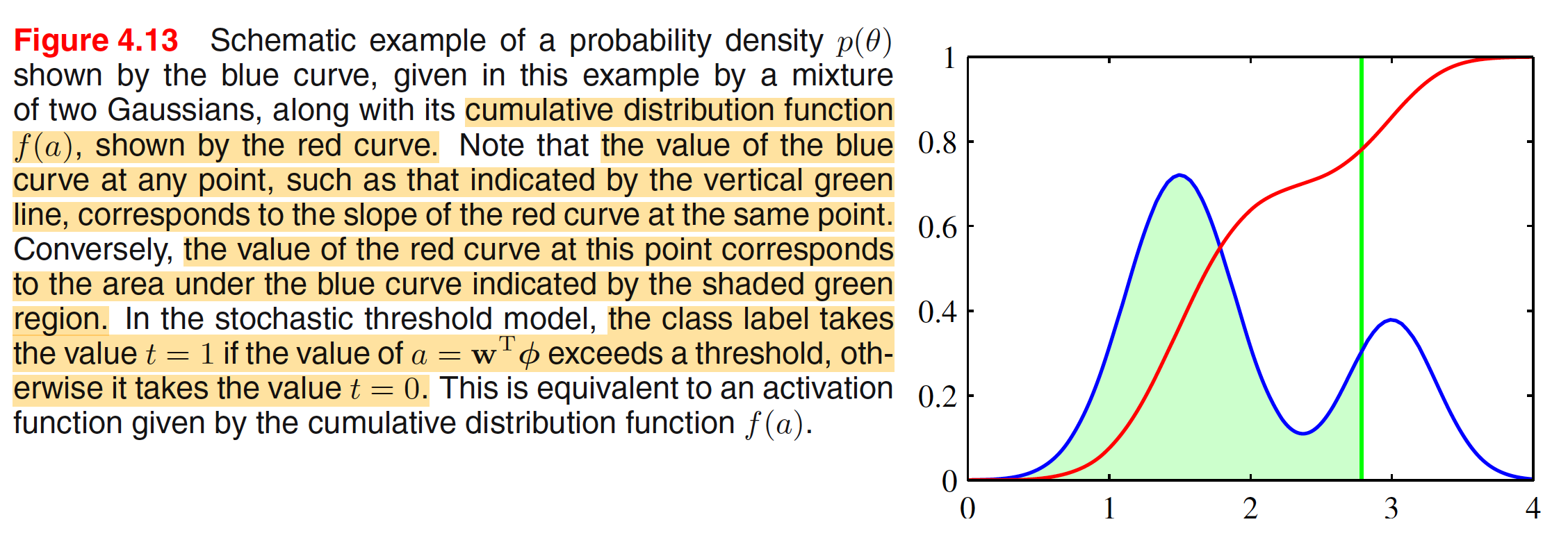
where $a_n = W^T_{n}\phi_n$. If the value of $\theta$ is drawn from a probability distribution $p(\theta)$, then the corresponding activation function will be given by the cumulative distribution function
$$\begin{align} f(a) = \int_{-\infty}^{a} p(\theta)d\theta \end{align}$$
This is illustrated in below figure.
Let $p(\theta)$ is given by $0$ mean unit variance Gaussian, i.e.
$$\begin{align} p(\theta) = \frac{1}{\sqrt{2\pi}} exp \bigg(-\frac{\theta^2}{2}\bigg) \end{align}$$
Corresponding cumulative distribution function is given as
$$\begin{align} f(a) = \frac{1}{\sqrt{2\pi}} \int_{-\infty}^{a} exp\bigg(-\frac{\theta^2}{2}\bigg) d\theta \end{align}$$
$$\begin{align} = \frac{1}{\sqrt{2\pi}} \int_{-\infty}^{0} exp\bigg(-\frac{\theta^2}{2}\bigg) d\theta + \frac{1}{\sqrt{2\pi}} \int_{0}^{a} exp\bigg(-\frac{\theta^2}{2}\bigg) d\theta \end{align}$$
$$\begin{align} = \frac{1}{\sqrt{2\pi}} \frac{\sqrt{\pi}}{\sqrt{2}} + \frac{1}{\sqrt{2\pi}} \int_{0}^{a} exp\bigg(-\frac{\theta^2}{2}\bigg) d\theta \end{align}$$
$$\begin{align} = \frac{1}{2} \bigg[ 1 + \frac{1}{\sqrt{2\pi}} \int_{0}^{a} exp\bigg(-\frac{\theta^2}{2}\bigg) d\theta \bigg] \end{align}$$
$$\begin{align} = \frac{1}{2} \bigg[ 1 + \frac{1}{\sqrt{2}} erf(a) \bigg] \end{align}$$
where
$$\begin{align} erf(a) = \frac{2}{\sqrt{\pi}} \int_{0}^{a} exp\bigg(-\frac{\theta^2}{2}\bigg) d\theta \end{align}$$
and the first integral can be evaluated by transforming $\int_{-\infty}^{\infty} exp(-{x^2}) dx = \sqrt{\pi}$. $erf(a)$ is known as the erf function or error function. The parameters of the model can be determined using the idea of maximum likelihood and is similar to those of logistic regression. In the presence of outliers, bothe the models vary differntly. The tails of the logistic sigmoid decay asymptotically like $exp(−x)$ for $x \to \infty$, whereas for the probit activation function they decay like $exp(−x^2)$, and so the probit model can be significantly more sensitive to outliers.